Chapter 29, Going nano (HSP Characterizations of Nanoparticles)

It’s obligatory to have a nano chapter because nano is new and exciting. In fact the truth is that nano is old and HSP have been solving nano issues for decades. We know this because the chapter on “insoluble” HSP is all about carbon black and carbon black has been nano ever since it first appeared as smoke.

But this chapter is a reminder that those working at the cutting edge of science could do well to remember older, simpler principles. We start with that great symbol of nano-modernity, the carbon nanotube, CNT.

Note. The following section was written before the work of Detriche et al (see below) was published. It is interesting to compare our predictions with those of the Detriche paper.

Although there are some papers that specifically invoke HSP for understanding the best solvents for dispersing CNT, we have found the data to be rather unsatisfactory. First, these papers don’t have a sufficiently full range of solvents to define the sphere in 3D. Second, we think that the data for good dispersion is skewed by high density or high viscosity liquids. Because the test for a “good” solvent is whether a dispersion remains stable over time, a high density or viscosity can give a misleading result. Ch.7 of the Handbook introduced the concept of RST – Relative Sedimentation Time – to help correct for differences in sedimentation due to density/viscosity:

RST=t_s(ρ_p- ρ_s)/ η

where t_s is the actual sedimentation time, ρ_p and ρ_s are the densities of the particles and solvent and η is the viscosity. The RST values should then be used to decide between “good” and “bad” solvents.

Happily a paper K.D. Ausman, R. Piner, O. Lourie, and R.S. Ruoff, Organic Solvent Dispersions of Single-Walled Carbon Nanotubes: Toward Solutions of Pristine Nanotubes, J. Phys. Chem. B. 104, (38), 8911-8915, 2000 gives a range of good solvents which, when combined with those known to be bad gives the following excellent fit:

 

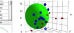
Figure 1‑1 Fit of Ruoff’s CNT data

The values aren’t too far from the less reliable fit which gave a value in the [18, 10, 9] region. The Solvent Optimizer readily informs us that DMF/Xylene (69/31) or Caprolactone/ Dipropylene Glycol Mono n-Butyl Ether (67/33) would be mixtures superior to any of the individual solvents used in the above experiment.

The paper by Detriche et al Application of the Hansen Solubility Parameters Theory to Carbon Nanotubes, J. Nanoscience and Nanotechnology, 8, 1-11, 2008 is an interesting vindication of the comments above. Although the paper covers many different types of CNTs, the data below are specific to Single Wall Nanotubes, SWNT.

First, they confirmed that without thorough centrifugation of dispersed samples results are highly unreliable as viscosity and density can skew the apparent solubility/dispersability of CNT. Their paper casts some doubt on some of the “good” solvents used in the fit above, which may partially explain differences between the two studies in the calculated values for CNTs.

Second, they showed that mixtures of two good solvents can give better solubility/dispersability. So a 50/50 mixture of o-dichlorobenzene/benzaldehyde gave a higher (8x) solubility than either alone.

	δD	δP	δH	Ra
SWNT	19.4	6.0	4.5	Radius=3
o-Dichlorobenzene	19.2	6.3	3.3	1.30
Benzaldehyde	19.4	7.4	5.3	1.61
50/50 mix	19.3	6.9	4.3	0.9

 

Third, and an excellent vindication of HSP principles, is the fact that a 75/25 mixture of two non-solvents gave a reasonable solubility

	δD	δP	δH	Ra
SWNT	19.4	6.0	4.5	Radius=3
Diethyl phthalate	17.6	9.6	4.5	5.1
Methyl naphthalene	20.6	0.8	4.7	5.7
75/25 mix	19.3	6.9	4.3	3.1

 

The authors had also noted a flaw in their initial study with 16 solvents. The chosen solvents did not give a sufficiently good bracketing of HSP space so the Sphere calculation could not produce a reliable fit. They could have used more solvents. But instead they used a large number of solvent mixes which, of course, achieves the

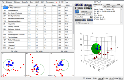
same thing. A plot of their 2 best single solvents gives the following:

Figure 1‑2 Fit of Detriche CNT data

If the “2” solvents are used then the result is meaningless sphere. But by using the mixture range they were able to bracket the CNTs and obtain the value shown in the table above.

Fifth, they recognised a further HSP principle – that larger polymers have smaller radii. They were able to fractionate CNTs using this principle – the average CNT size in a “good” solvent was considerably smaller than the size in a “very good” solvent.

Sixth, though it hardly needs pointing out, Hildebrand parameters proved a poor way of predicting solubility behaviour.

Surfactants are also a popular method for obtaining good dispersions of CNT in water. So far we have not been able to find a good correlation between the HSP of the surfactants and their dispersion capabilities for the CNT. The standard hydrophile/hydrophobe chains in these surfactants simply don’t seem to have the capability of producing HSP with the required high δP and δH.

Two papers from the Coleman group explicitly use HSP to further push the boundaries of CNT and graphene solubilities. Shane D. Bergin, Zhenyu Sun, David Rickard, Philip V. Streich, James P. Hamilton, and Jonathan N. Coleman, Multicomponent Solubility Parameters for Single-Walled Carbon Nanotube Solvent Mixtures, ACNano, 3, 2009, 2340-2350 and Yenny Hernandez, Mustafa Lotya, David Rickard, Shane D. Bergin, and Jonathan N. Coleman, Measurement of Multicomponent Solubility Parameters for Graphene Facilitates Solvent Discovery, Langmuir, DOI: 10.1021/la903188a. The HSP analysis (the authors used HSPiP during their research) is not perfect and doesn’t explain everything, but such huge “molecules” really are pushing the boundaries of HSP. Nonetheless, it’s clear that HSP do a quite impressive job in helping understand these complex phenomena.

Similarly, recent work from the Delhalle group throw more insight into CNT surfaces, especially the fact that many “functionalised” CNT are very poor mixtures of undefined quality. See Detriche, S., Nagy, J.B., Mekhalif, Z., Delhalle, J, Surface State of Carbon Nanotubes and Hansen Solubility Parameters, Journal of Nanoscience and Nanotechnology, 9, 2009 , 6015-6025.

C60

We can’t miss the chance to discuss C60. There have been numerous attempts to understand the slightly odd solution behaviour of C60. Not many other chemicals are best dissolved in chloro- or phenyl-naphthalene at room temperature. Many efforts using QSAR techniques sifted from 1000’s of possible “molecular” properties have produced correlations with R² from 0.6 (poor) to 0.9 (not bad), but with little apparent insight into what is really going on. Hansen and Smith used basic Sphere techniques in their paper C.M. Hansen, A.L. Smith, Using Hansen solubility parameters to correlate solubility of C60 fullerene in organic solvents and in polymers, Carbon, 42 (2004) 1591–1597 to find HSP of [19.7, 2.9, 2.7] and thereby to make predictions of 55 solvents that might do a reasonable job and then went on to show which polymers (polystyrene is a good example) would have good compatibility with C60.

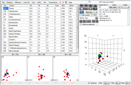
We’ve taken advantage of a rather expanded data set to re-do the correlation. Here is the Sphere with 107 solvents instead of the original 87. The definition of good “1” solvents is Log(MoleFraction)>-3.0.

Figure 1‑3 Fit of Hansen C60 data

The result is [20, 3.2, 2.0] which is close to the original fit. If the definition of “good” solvents is changed to include all the “2” solvents, defined as Log(MoleFraction)>-4 the value changes to [20.5, 3.8, 1.6], only a modest change.

Because there is such a tradition of doing least-squares fits of the Log(MoleFraction) data, we did the same, using the formula:

Log(MoleFraction) = K * Sqrt(4*(δDc60-δDs)² + (δPc60-δPs)² + (δHc60-δHs)²)

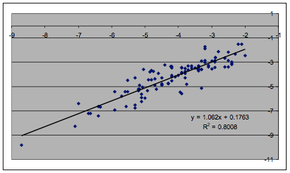
Figure 1‑4 Least squares fit of Hansen C60 data

 

The R² is a respectable 0.8 when the C60 HSP are set to [22.5, 0.6, 2.9], remarkably close to the Sphere fit.

Of course there’s more to solubility of a molecule like C60 than enthalpy. There must surely be some entropic effects and, presumably, some specific inter-molecular effects. But straightforward HSP do a remarkably good job at covering this large range of solubilities and, importantly, provide practical predictions on solvents and polymer compatibility that the working scientist can combine with intuition and experience to help develop processes for C60. The fit is close to the best published fits via QSAR without the need for those 1000+ factors available to practitioners of that art. The bottom line is that C60 is in an awkward position in solubility space – not many liquids have δD values in the 20+ range and even less combine that with low δP and δH values. Chemicals with such high δD values are (usually) solids. It’s the δD which makes it so hard to find convenient solvents for processing C60, it’s as simple as that.

And for those who wish to test out a prediction. From published data of cohesive energy density, sulphur comes out with a value in this high δD range so it’s probably a good solvent if you wish to try it.

Graphene too

The amazing properties of graphene hold great promise for many applications. Geim’s initial method for producing it using adhesive tape is breathtakingly simple and inspired but not adequate for mass production. 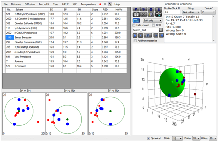The paper by Coleman and his large team, High-yield production of graphene by liquid-phase exfoliation of graphite, Nature Nanotechnology, 3, 563-568, 2008, shows that graphene is soluble in a solvent as simple as Benzyl Benzoate and therefore potentially graphene coatings can be produced direct from solvent. We’ve plotted their data (with their permission) in HSP terms and obtained the following value for the HSP of graphene:

Figure 1‑5 Fit of Coleman’s Graphene data

 

When [20, 11.2, 7.3] is put into Solvent Optimizer, a near-perfect match is obtained by a 60:40 blend of Caprolactone and Benzyl Benzoate. It will be interesting to know if this blend is actually better than Benzyl Benzoate alone.

Nano-clays

Clays are remarkably cheap and, with a bit of exfoliation, are remarkably nano. A lot of people have therefore spent a lot of time trying to make polymer/clay nanocomposites. With hindsight it is clear that a lot of this work has been wasted because, first, exfoliating the clays is not easy and, second, it is not obvious which organic groups would be most compatible with a given polymer.

The best-known method for aiding exfoliation is to create an organoclay via ion exchange to remove the sodium ions between the plates and replace them with a quaternary ammonium salt, typically containing a mixture of methyl, benzyl, hydroxyethyl and tallow groups. If this is done well then the resulting clay contains neither excess sodium nor excess quaternary salt. But doing things well makes the clays more expensive. But by using impure versions, interpreting the data is very difficult.

Assuming the organoclay is of high quality, what is the best one to use for any given application? Usually the ideal is total exfoliation of the clay within the polymer. But many users are happy if they have lots of “tactoids” (nano clusters of clay particles) which are, at the very least, better than mechanically dispersed clay microparticles.

At this stage it would be good to show that HSP can come to the rescue.

Unfortunately, the data don’t allow the production of good HSP. The file Clay4 fits the data from D.L. Ho and C.J. Glinka, Effects of Solvent Solubility Parameters on Organoclay Dispersions, Chem. Mater. 2003, 15, 1309-1312. The clay is dimethyl-ditallow montmorillonite (Cloisite 15A) and gives an HSP set of [18.2, 3.8, 1.7]. Unfortunately, attempts to fit (nominally) the same clay from the data of D. Burgentzlé et al, Solvent-based nanocomposite coatings I. Dispersion of organophilic montmorillonite in organic solvents, Journal of Colloid and Interface Science 278 (2004) 26–39, shown in Clay2, gives the impossible values of [16.8, -4.7, -3.3]. The problem is compounded by the fact that the solvent data contains its own uncertainties. Does one class as “good” solvents those that swell the clay or those that cause a big increase in the interlayer spacing? Furthermore, one of the really good solvents in the first paper, chloroform, is a bad solvent in the second.

From the second paper, the dimethyl-benzyl-tallow (Clay1 – Cloisite 10A) gives [20.4, 6.6, 5.9]

 

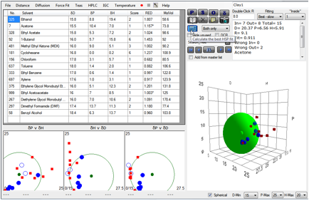
Figure 1‑6 Clay 1 fit

and the methyl-di(hydroxyethyl)-tallow (Clay3 – Cloisite 30B) gives [15.8, 15.2, 11.0]. Adding n-alcohol data from another paper on the 30B gives [16.7, 10.4, 10.2], though there is a contradiction with the data point for ethanol.

Because organoclay nanocomposites look to be of such great importance it would seem a good idea to re-test the solvent swelling data on a group of well-defined clays, using a larger range of solvents across HSP space to gain a better set of values or, conversely, to show that for some reason the HSP approach is not appropriate.

Nevertheless, when one of us (Abbott) tried applying the HSP data to a group of papers on organoclays in poly(lactic acid) [18.6, 9.9, 6.0], it became obvious that the popular 30B was less likely to be a good match than the 10A, whilst the also much-used 15A was likely to be unsatisfactory. The revised data on 30B reduced the degree of mismatch with the poly(lactic acid) – re-emphasising the need for a definitive data set on these clays.

Recent work by a team led by Dr Andrew Burgess (then in ICI, now in Akzo Nobel) gives some visual elements to this story. We are grateful to Dr Burgess for permission to use their material here. They used a set of Cloisite clays and attempted to disperse them in a range of solvents. Typical results for four solvents are shown:

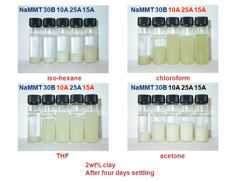
Figure 1‑7 Some of the data for Cloisite clay dispersions from A. Burgess, D. Kint, F. Salhi, G. Seeley, M. Gio-Batta and S. Rogers, reproduced with permission.

 

For example, it’s clear that chloroform is good at dispersing/swelling 10A, 25A and 15A, whilst THF is only good for 10A and 15A. i-Hexane and acetone don’t do a good job with any of the clays. From their full dataset they tried an analysis using Hildebrand solubility parameters. The results were unconvincing. The same data put into HSPiP allowed a more insightful analysis. Here, for example, are the data for the Cloisite 10A:

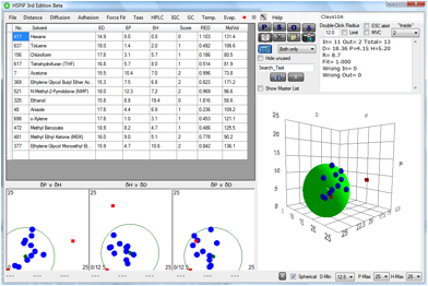
Figure 1‑8 A fit for the Cloisite 10A results from Burgess et al.

As the files are provided with HSPiP you can judge for yourself how good or bad the fits are. A larger range of solvents would, as always, provide greater certainty. But a retrospective analysis of the Burgess’ team’s attempts to combine the clays with various common acrylates showed that the HSP were a good indication of the relative ease or difficulty of making stable clay dispersions.

 

Quantum dots

When a particle of something as ordinary as CdTe becomes smaller than ~10nm then its electronic properties are governed by the wave function that can fit inside the dot rather than the properties of the material itself. So CdTe can become green, red or blue depending on the particle size. There are numerous applications for such quantum dots. But because small particles have large relative surface areas they tend to clump together, losing their quantum-dot nature and/or their ability to be dispersed in the medium of choice.

Because there are so many different quantum dots, stabilised by a large variety of different methods, there seems to be no general theme emerging for which HSP give an over-arching insight. However, one data set kindly provided to us by Michael Schreuder working in Professor Rosenthal’s group at Vanderbilt University shows a mixture of the expected and the unexpected. CdSe nanocrystals were stabilised with a shell of a substituted phosphonic acid. Here is a typical example of a fit with 43 solvents for the Butylphosphonic acid system:

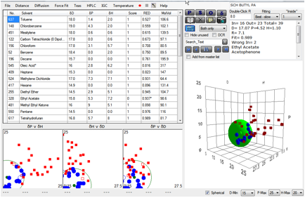
Figure 1‑9 The fit to a Quantum Dot

 

The calculated values [17.0, 4.5, 1.1, 7.1] seem reasonable for a somewhat polar butyl chain. The problem is that when one goes to the phenyl phosphonate, the values are remarkably similar. The fit of [16, 4.7, 2, 5.3] has a disturbingly low δD value. The fit for the Octylphosphonic acid version [17, 3.7, 1.5, 6.8] does not show the expected decrease in δP and δH for the longer alkyl chain. And, surprisingly, the 2-Carboxyethylphosphonic acid fit [16.4, 4.8, 3.2, 4.7] shows no evidence for the expected higher δP and δH. Even worse, some of the fits (not included, for reasons we’ll describe in a moment) were very poor quality.

But maybe we are jumping too quickly to conclusions. We’re assuming that the CdSe surface is entirely covered by a shell of substituted phosphonic acids, with the chains sticking out into the solvent, so the HSP should be that of the chains. But what if some of the CdSe, or the phosphonate group is accessible to the solvent – how much would that contribute to the HSP? Conversely, what would happen if there were still an excess of the phosphonate – that would give strange results. The investigators checked out this last possibility. The samples that gave poor results were checked using Rutherford Backscattering and were found to contain excess phosphonate. At the time of writing, the reason for the relatively uniform HSP for the range of phosphonates has not been found, but it is satisfying to note that when some poor fits suggested either that the HSP approach was wrong or that the samples themselves had issues, it was the latter that was found. This does not prove that HSP are right, but once again it shows that they can be deeply insightful even down to the level of quantum dots.

 

E-Book contents | HSP User's Forum