For more than 40 years the Sphere technique has been used with great success. But sometimes you don’t quite have the solvent you need so you add one or two pseudo-solvents created via the mixing rule. So if you don’t want to use dimethyl formamide in a test you can create something close (using the Solvent Optimizer) with, say, a 60:40 mix of DMSO and THFA. This technique has been used numerous times.

But why stop there? Why not make a whole Sphere test from mixed solvents? If, for example, 3 pairs of solvents covered the range of interest then instead of finding 20-30 different solvents, you can stock just 6 of them, and if you have a robot it’s rather efficient to make up the set of possible blends from the 3 pairs of those 6 solvents.

Although others may have done this before, the Brabec group at U. Erlangen have shown how powerful the technique can be in a paper that tried to narrow down the HSPs of materials used in organic photovoltaic systems:  Determination of the P3HT:PCBM solubility parameters via a binary solvent gradient method: Impact of solubility on the photovoltaic performance, Florian Machui, Stefan Langner, Xiangdong Zhu, Steven Abbott, Christoph J.Brabec, Solar Energy Materials & Solar Cells 100 (2012) 138–146.

The technique seemed so powerful that for HSPiP it was termed the Grid method (because it assembles a grid of points throughout the 3D space). The initial version of the Grid was highly experimental but rapidly proved so popular that it has been expanded, with the ability to create a Grid automatically from a list of chosen solvents.

An example using the Default set is shown:

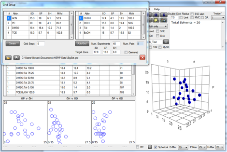
Figure 0‑1 A Grid based on the Default set

In this example 4 pairs of solvents are chosen: Acetonitrile:Cyclohexanol; Propylene Carbonate:Ethanol; DMSO:Toluene; Tetrachloroethylene:Butanol. Abbreviations are used because, as can be seen from the main form, the individual points are made up of the step-wise variation of the pairs and their full names would over-fill the space for the names.

This particular grid is chosen because it rather effectively fills a large part of HSP space. But of course it is not perfect. There are some significant holes in that space. But the point of the Grid is that it is entirely flexible. You can fill those holes by changing the pairs or you can add a few specific single solvents. It is your choice.

This sort of Grid is general purpose. An alternative, which is equally powerful (and is the choice in the Erlangen paper) is to start with a single good solvent and explore the Sphere in 3 directions.

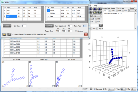
Figure 0‑2 A Grid using a single solvent (hopefully) at the centre of the Sphere

Here the idea is that the material of interest is soluble in DBE and by scanning out in 3 different directions the radius and (probably) the centre can be defined more precisely than tends to happen with the usual assortment of solvents.

One user loved the idea but wanted to be able to create Grids automatically from a chosen set of solvents which happen to be the only ones usable (for cost, tox, volatility reasons) in their area. So the AutoGrid method takes a selected list of solvents (from the Solvent Optimizer) and a Target Zone of interest and attempts to create a suitable Grid. Finding a perfect algorithm for this has proven difficult, but it seems that the choice of solvents is even more important than the choice of algorithm. If, for example, Hexane:MEK turns out to be a good scan line within the Grid, then Heptane:MEK would also be a good scan line. If the solvent list contained both Hexane and Heptane then the chances are that both lines would be included in the Grid (because they are both “good”), adding nothing whatsoever to the quality of the resulting data. Although in principle a smart algorithm can remove such pseudo-duplicates, given that humans are smarter than computers it’s a good idea just to include heptane as it’s usually rated less toxic than hexane.

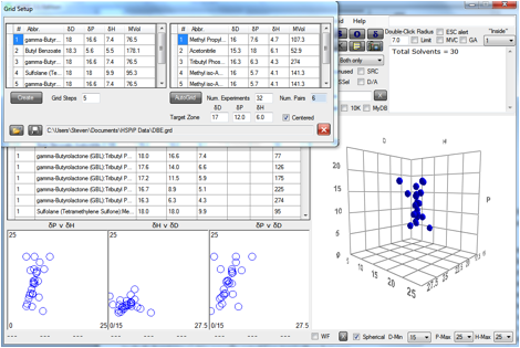
Figure 0‑3 An AutoGrid aimed at the [17, 12, 6] zone

This particular AutoGrid is limited to 32 experiments, so at 5 steps/scan-line, that means 6 pairs of solvents. The “Centered” option was chosen to force the lines to cross the sphere as much as possible. No doubt a human could come up with a better Grid from the given set of solvents, but it would take much longer and at least the automated version offers a starting point for human intervention.

A question that is often asked is: “How good are mixed solvents compared to the same HSP from a single solvent?” The answer from experiments carried out over 40 years is “In HSP terms they work very well, but in kinetic terms, and in situations where entropic effects are important they act as if they were a solvent with a larger MVol”. So if in the example at the start DMF was a fast solvent for polymers, the DMSO:THFA mix would be rather slower. And because entropic effects are important in polymer solubility, the mix would not give as high a solubility as the single solvent.

This means that the Sphere radius from mixed solvents will be rather smaller than if it had been measured with single solvents. For most users, the ease and convenience of the Grid and the chance of a more accurate Sphere centre seem to outweigh the issue of a potentially smaller radius.

E-Book contents | HSP User's Forum