Chapter 6, Safer, Faster, Cheaper (Optimizing Solvent Formulations)

With the Optimizer you can quickly home in on the HSP of your target. Let’s assume, as in Coming Clean, that we want to dissolve a polymer in an ink. If we know that the polymer has HSP of [18.6, 10.1, 7.8] then we can use HSP tables to find the best match. From a large list you can find that N-Acetyl Piperidine and Hexamethylphosphoramide are excellent matches, but you are not likely to want to use either of those!

Out of your 19 solvents, the RED number shows you that N-Methyl-2-Pyrrolidone is not a bad match, but it’s expensive, slow to evaporate and has some health & safety issues.

It looks as though we’re stuck. But remember that a solvent blend with the same parameters as the polymer is thermodynamically identical to a pure solvent. So if we can’t find the perfect single solvent, let’s find a blend.

If you’ve ever tried doing this manually from a list of solvent HSP you will know that it’s a bit of a slog. So let’s get the computer to do it.

The Optimizer comes with a list of “friendly” solvents – ones that you might find in general use and which aren’t too toxic or expensive. Everyone’s definition of “friendly” differs so you should feel free to modify the list for your own purposes.

When you enter the Target HSP (in this case [18.6, 10.1, 7.8]) you can then select one or more solvents and their % and click the Calculate button to compute the HSP of the blend – which is simply the weighted sum of the individual components. The Distance is also automatically calculated – the smaller it is, the better.

This is helpful for scouting purposes but it is hard to find an optimum this way.

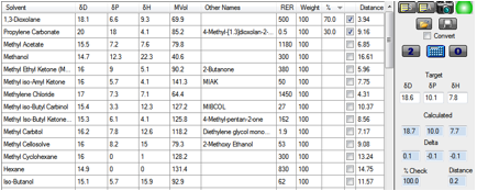
A quick short-cut is to click the 2 button which does an exhaustive search of all possible combinations of 2 solvents to find the closest match (smallest Distance). When we do this, a blend of 1,3-Dioxolane and Propylene Carbonate is chosen.

 

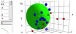
Figure 1‑1 Solvent Optimizer trying to match the polymer’s [18.6, 10.1, 7.8]

This will undoubtedly be a fast dissolving blend. Both molecules have a small Molar Volume (MVol) and small means fast diffusing (kinetics) and large entropy change (thermodynamics) for good dissolution.

So we have Faster. But what about Safer? The flash point of 1,3-Dioxolane is rather low so you might not like to include it. If you go into the main program and load the full set of solvents you can do the “Double Click” trick on 1,3-Dioxolane to find that Tetrahydofurfuryl alcohol is not too far away from it. That is certainly not too volatile. So let’s deselect the Dioxolane and select the alcohol. What % should be used? The simplest way to find out is to click the Optimize button. It turns out that a 75:25 mixture is optimal. The Distance is a bit larger, but it should still be OK. The MVol is also OK. So now we have Faster and Safer. Unfortunately, Tetrahydofurfuryl alcohol is rather expensive. So we have to work a bit harder to get Cheaper. By exploiting some Advanced Optimization tricks within the Optimizer it’s possible to find that a combination of Dipropylene Glycol (DPG) and Aromatic Hydrocarbons is not a bad match for Tetrahydofurfuryl alcohol. So now we click the Optimizer button once more and find that we have got a good blend of Faster, Safer and Cheaper with these 3 solvents:

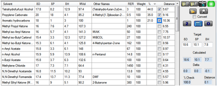
Figure 1‑2 A blend optimized by clicking the O button

Of course there are always trade-offs. This blend has the relatively high MVol of the DPG so Faster has been compromised – but if this is a priority then you can carry on searching in a rational manner to replace the DPG with something smaller.

For those who wish to avoid Aromatic hydrocarbons it’s possible to find blends of 4 or 5 components that do a good job. We leave that as an exercise for the reader.

Let’s remind ourselves what we’ve done in such a short time. With 16 simple tests of whether a solvent dissolved or didn’t dissolve our ink we found the HSP of the ink. We did 3 more tests just to refine the value. Then after about 30 minutes on the computer we found a 38:33:29 mix of Propylene Carbonate, Aromatic hydrocarbons and DPG as a Faster, Safer, Cheaper blend. Can you imagine how long it would have taken you to find such a blend without HSP?

It’s no coincidence that solvents with this sort of mixture of aromatics, propylene glycols and high P solvent are widely used in the “safer solvents” industry. Indeed, one of us (Hansen) helped found a Danish “safer solvents” business on the basis of patents derived from the insights of HSP.

When in doubt go higher

If you had a choice of two solvents, the same distance from the target, and one is of low δTot and the other is of high δTot, which one should you choose? Hansen’s view is that higher is better. Why? The analogy is with the Kauri Butanol number. A “poor” solvent causes the kauri to crash out after relatively little dilution, a “good” solvent is tolerated to a much greater extent. Because (by definition) butanol is used in the test, high δTot solvents are likely to be more compatible with the butanol and therefore limit the crashing out of the kauri. Armed with HSPiP one could probably find plenty of exceptions to this rule of thumb, but to the extent that the Kauri Butanol number is of any value (and that’s debatable) the “higher is better” rule is a reasonable guide.

Squared mixing algorithm

For the past 40 years, the simple weighted volume average discussed above has proved to be an acceptable way to formulate. However, an argument can be made that a “squared mixing algorithm” should be used. For example, if solvent 1 and solvent 2 are present in volume fractions of x and y then each δ of their mixture would be:

δ_mix= sqrt(xδ₁² + yδ₂²)

Because this is cumbersome to apply it’s seldom been used. For the 3^rd Edition we have added the option. We will be very interested in user feedback on whether it is, in fact, superior to the linear algorithm. For modest differences in δ the two algorithms give results within the usual margin of error; the algorithms only diverge significantly when there are very large differences in δ.

In the next chapter we show how HSP can make the incompatible, compatible.

 

E-Book contents | HSP User's Forum