Chapter 16, HSP and Diffusion 

Diffusion of chemicals through polymers is a highly complex and highly debated issue. In this chapter it is shown that HSP offer profound insights into these phenomena. Diffusion in polymers as such is not directly connected to thermodynamics (HSP) but instead has a lot to do with kinetics. There are (at least) two reasons for facing up to the controversy with the help of HSP. The first has to do with Health & Safety. As other chapters show, HSP have a lot to offer on the subject of protective workwear such as gloves. The second reason is that diffusion lets us tackle head on the thermodynamics v kinetics controversy that often gets in the way of the use of HSP.

The good news is that although the calculations of diffusivity are rather hard to implement, the theory of what is going on is remarkably simple. A diffusion modeller is included within the HSPiP package so you can explore the theory without having to worry about its detailed implementation. In what follows we are referring only to solvent diffusion under constant temperature and are not discussing diffusion driven by other gradients such as temperature.

For those who just want a quick method to estimate diffusion coefficients, the official Nordtest Poly 188 found at http://www.nordicinnovation.net/nordtestfiler/poly188.pdf gives a well-validated methodology that is a simplified version of what is found in this chapter. It is no coincidence that Hansen was one of the authors of the Poly 188 test.

Contrary to popular mythology, there is only one type of diffusion that is important for polymers in normal practice. If you do practical experiments you might be surprised by this statement because it’s rather obvious that there are at least two distinctly different situations of interest: absorption (solvent going into a polymer) and desorption (solvent coming out of a polymer). This is obvious to anyone who has done absorption/desorption experiments because absorption is generally much faster than desorption. Those of you who know more about the topic will also be aware that some diffusion rates are simple (“Fickian” diffusion) and some are complex (e.g. “Type II” diffusion).

The response to this apparent complexity is to repeat that there is only one type of diffusion based on just one simple equation, the diffusion equation (sometimes called Fick’s second law). The apparent differences between all the different types reflect the fact that different factors involved in this equation are more or less important depending on circumstances. The reason to stress this simple unity is that each of the different factors is rather easy to understand. It is therefore rather easy to work out which factors are required to sort out what is happening in just about any diffusion behaviour. Armed with HSP of solvent and polymer, with some knowledge of molar volume (integral to HSP) and molecular shape, and with some understanding of whether (and when!) a polymer is highly crystalline, semi-crystalline or elastomeric (often reflected in the HSP Radius), you can readily calculate diffusion behaviour. As discussed below, the diffusion rate increases in the order highly crystalline < semi-crystalline  < elastomeric as governed by Factor 5. These categories are gross simplifications only to be used as rules of thumb – there are certainly cases of crystalline polymers with higher diffusion rates than semi-crystalline. But these rules are a good starting point. We provide some more rules of thumb on diffusion rates in the text and in the HSPiP modeller.

Consider the following factors, one by one.

Factor 1. This is the Mass Transfer Coefficient, h. A large h means that if you have a well-stirred liquid in contact with the polymer surface then you have no shortage of molecules to be able to diffuse into the polymer. If, on the other hand the polymer surface is in contact with still air, then a boundary layer builds up and solvent trying to escape from the polymer will see a high concentration of vapour which reduces the gradient for diffusion and therefore slows down the rate, so h is small. One reason for there being a difference in absorption and desorption in this case is the simple and obvious fact that the Mass Transfer Coefficient from 100% liquid in absorption is much higher than that into a boundary layer of air (saturated with vapour) in desorption. But there also can be times when mass transfer into the polymer from a liquid is limited (e.g. poor stirring of an inert carrier liquid such as water, with fast absorption of a solute). In all of these cases there is rapid diffusion of the chemical within the polymer and some problem with mass transport more or less exterior to the polymer.

Another factor which can cause large reductions in the mass transfer coefficient is the formation of a highly-crystalline skin at the surface. The absorbing molecule simply cannot find any access point into the bulk (less-crystalline) polymer. The reduction in mass transfer coefficient is larger for larger and/or more complex molecules. Above a certain size the mass transfer coefficient becomes zero – there is no penetration into the bulk. The most extreme example of this is when two polymers, even well-matched in terms of HSP, simply cannot interpenetrate. What is surprising is that even some simple molecules (e.g. a single benzene ring or a modestly branched structure) can have a mass transfer coefficient close to zero for some polymers such as those with high crystallinity or other forms of close-packing such as are found in the Topas polymers. Chapter 16 of the Handbook discusses some of these issues in greater detail.

A good method for checking if diffusion is limited by mass transfer is to carry out the experiments on samples of different thicknesses – the thicker the sample, the less relevant the mass transfer effect becomes – as you can readily determine using the diffusion modeller.

Given that most of us don’t know what the Mass Transfer Coefficient is for our systems, the modeller uses the Hansen B value. This is the ratio of the diffusion resistance to the surface resistance. With D₀ as the diffusion coefficient at the lowest concentration encountered, and for a free film sample of thickness L, the diffusion resistance is (L/D₀). Dividing this by the surface resistance (1/h) gives B. Thus,

B= hL/D₀

A high B (>10 for a constant diffusion coefficient) means essentially no significant limitation by mass transfer.

Factor 2. This is the local saturated concentration of the liquid in the polymer right at the surface during absorption. For RED less than 1 for a correlation based on “good” or “bad” solubility, this concentration will be very high since the solvent can in principle completely dissolve the polymer. It is very difficult to assign an initial given surface concentration, but it is probably in the range of 50-70%, because at still higher concentrations, the issue is not one of diffusion of solvent into the sample but diffusion of the sample into the solvent. For RED larger than 1, the larger the value, the lower the local saturated concentration and therefore the slower the absorption rate. This is the reason that HSP is so important for understanding diffusion. In the modeller a simple algorithm has been used to illustrate this so you can compare overall diffusion rates as the RED changes. The algorithm is for illustrative purposes only – it’s up to you to specify the surface concentration in any specific scenario.

Once the molecule is inside the polymer, as long as it is within its solubility limit (we’ll explain this in a moment), HSP play no further role. The rates of diffusion of a low RED and high RED solvent of similar molar volume and shape are the same. You might be surprised that in an HSP book it is claimed that HSP are not important for diffusion inside the polymer, i.e. the diffusion coefficient at a given concentration. The experimental data have confirmed this fact many times. This also means that HSP play no part in classic desorption experiments to air. Naturally the desorption from one polymer to another (migration) does depend on the HSP of the second polymer as a large HSP mismatch would mean, as in absorption, a low surface concentration in that polymer.

Although Factor 2 is about absorption, it’s a good point to discuss why desorption takes so much longer than absorption. It has been shown that the diffusion coefficient increases exponentially with the concentration of the solvent. For rigid polymers this increase is a factor of about 10 for each 3%v increase in solvent concentration. For flexible polymers the increase is a factor of 10 for about 15%v increase in solvent concentration. Whereas during the whole time of the absorption process, the solvent is largely diffusing in at concentrations approaching the maximum (surface equilibrium) concentration, and certainly much higher than the lowest concentration, in desorption most of the solvent diffuses out at much lower (and falling) concentrations than the initial one. In desorption the concentration at the surface is low (zero) so the process is largely controlled at or near the exit surface since the diffusion coefficient here is so low.

Before going to Factor 3, let us clarify this statement that “as long as it is within its solubility limit, HSP play no further role.” If you dip some polymers (e.g. epoxies or polypropylene) into hot water, the solubility is increased sufficiently for water to diffuse in (the δH of water falls off rapidly with temperature, boosting its solubility). If you then cool the sample, the water becomes insoluble in the polymer. The individual water molecules can still diffuse (diffusion coefficient is independent of HSP) but when they meet each other, they phase separate from the polymer. This is the classic case of water blisters. If you hot-dip/cool a number of times you get more and more water into the polymer, but each time you cool, the water phase separates out into bigger and bigger blisters. The blisters are very persistent. That is because each blister is a new diffusion problem from one phase (the water blister) into the other (the polymer). Given that there is a large HSP mismatch, the surface concentration at the blister/polymer interface is low so the rate of diffusion is low. Those blisters can be very persistent. So now you can see why it’s important to qualify the statement that HSP have no effect on diffusion once the molecule is inside the polymer. See p141 of the Handbook or C.M. Hansen, New Developments in Corrosion and Blister Formation in Coatings, Progress in Organic Coatings, 26, 113-120, 1995 for further details. Incidentally, a beautiful demonstration of HSP co-solvent effects is provided by the well-known fact that glycol ethers in coatings can produce blisters under aggressive thermal/water cycling tests. The ethers remain in the coating and during the hot/wet part of the cycle the combined glycol ether/water HSP is a sufficient match to the hot polymer to allow the water to enter. On cooling the blisters start to form. The same coatings without the glycol ethers have no blistering because the HSP distance of the water is too great, even at the higher temperatures.

Factor 3. This is the molar volume. The larger the molar volume, that is, the size of the molecule, the smaller the diffusion constant. This is a generalisation that is modified by Factor 4, and therefore it must be used as a guideline rather than a hard fact. In the modeller the rule of thumb (based on the rather small number of studies in the literature) is used that the log of the diffusion constant is proportional to the molar volume. The constant of proportionality changes strongly from rigid to flexible polymers. For rigid polymers there is a very strong dependence, so a doubling of molar volume can result in a 10 to 100-fold reduction in diffusion constant. For flexible polymers the dependence is weak – a doubling of molar volume may merely halves the diffusion constant.

Factor 4. This is the molecular shape. A linear, flexible molecule can easily wiggle through a polymer. A rigid (aromatic) molecule or a highly branched molecule takes much longer to find a space (or “free volume” – see Factor 5) in which to wiggle. The rule of thumb section below gives some examples of the effects of Factors 3 and 4. A well-known table of solvent diffusion rates from Shell suggests that the combined effects of molar volume and molecular shape result in a diffusivity order from faster to slower of: Methanol, Acetone, MEK, Ethyl Acetate, n-Heptane, n-Butyl Acetate, Benzene, 1,4-Dioxane, Toluene, MIBK, i-Butyl Acetate, 2,4-Dimethyl Pentane, Cyclohexane, Diacetone Alcohol, Pentoxone, Methyl Cyclohexane, Cyclohexanone, Methyl Cyclohexanone. This table was derived using the technique originally developed by Hansen when he created the data of Fig 1 of the chapter on glove data.

Factor 5. Informally we can say that Factor 5 is whether the polymer is rigid (slow diffusion), flexible (faster diffusion), or a quasi-solution – e.g. an elastomer where the polymer is held together by just a few crosslinks (still faster diffusion). More technically we can talk about polymer “free volume” where the rigid polymer is below its glass transition temperature (Tg) and therefore has little main-chain segmental motion and the flexible polymer is either naturally above its Tg or has large free volume for main-chain segmental motion thanks to all the solvent. It is Factor 5 which causes most of the confusion about diffusion science. The more free volume there is, (or, equivalently, the lower the glass transition temperatures), the faster will be the rate of diffusion. The simple view of all this is that when the solvent enters a polymer it starts to plasticize it and diffusion is faster. As more solvent diffuses into a polymer the diffusion rate can increase by factors of 100’s, 1000’s and even millions (the solvent itself is increasing the polymer free volume) so the diffusion looks more complex. This “concentration dependent” diffusion is not some sort of special case or special phenomenon – it is the general rule for polymers. Sometimes it looks “special” because the concentration dependence is so large – but this is only because the polymer happens to be rigid and therefore susceptible to a large increase in diffusivity. This simple view needs to be treated with caution. Some crystalline regions are so impenetrable to solvents that they act as permanent blocks so there is little increase in diffusion coefficient. Some “amorphous” polymers are in fact highly rigid so show a large increase in diffusion rate whilst others are highly flexible and therefore show a small increase. The following figure is for diffusion of chlorobenzene in polyvinylacetate.

 

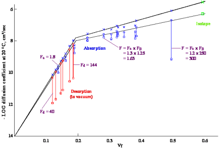
Figure 1‑1  Diffusion coefficients for chlorobenzene in poly(vinyl acetate) at 23°C measured by absorption and desorption experiments in a quartz balance apparatus as well as with an isotope technique. v_f is the volume fraction. The upper curve in the figure is for diffusion coefficients based on total film thickness. The lower curve is for diffusion coefficients based on dry film thickness as used in the modeller. It should be noted that the lower curve varies more and more from the upper one as the concentration of solvent increases. A self-diffusion coefficient for a liquid (vf = 1.0 in the figure) is a fictitious quantity on the lower curve, although it is used to define the diffusion coefficient in the solvent rich regime.

The data in the figure are the result of combination of absorption and desorption experiments supplemented by isotope experiments to give a unified view of concentration dependent diffusion in polymers. In every measurement the observed diffusion coefficient was initially considered as a constant that must be adjusted to the change in concentration within the film during the whole process. Solutions to the diffusion equation with different concentration dependencies were generated and compared with that for a constant diffusion coefficient to develop these “F” factors. The apparent, constant diffusion coefficients are given by squares in the figure with the corrected values being given by circles. The adjustments are for absorption, desorption, or surface effects as indicated by the subscripts a, d, and B. Desorption experiments take place largely at local concentrations within the film that are much lower than the initial concentration that is ascribed to the experiment. These adjustments are much larger for desorption than for absorption. The correction for surface effects in the absorption experiment at v_f = 0.5 is a multiplier of 250. Such experiments should not normally be used to measure diffusion coefficients at these intermediate concentrations. The procedure used for these adjustments is described in more detail in the Handbook. The upper curve is for diffusion coefficients based on the wet film thickness, while the lower curve is for dry films. It is clear that there are two different regimes, rigid at lower concentrations, and elastomeric at higher concentrations, separated by the break at about 0.2 volume fraction of chlorobenzene.

Diffusion coefficients at very high solvent concentrations are usually best described based on total film thickness rather than dry film thickness, since the value for the latter at zero polymer concentration becomes meaningless. A value at 100% liquid is required to define the diffusion coefficient curve, however, and this value will be somewhat lower than that found in the literature for self diffusion in the given liquid. Fortunately, diffusion at very high solvent concentrations is usually so rapid as to not be a significant effect in the situations of major interest, so smaller deviations in this region are not important. Whether diffusion is very rapid or “super-rapid” does not really matter since the process is controlled by what happens at (much) lower concentrations. Usually the surface concentrations at equilibrium for absorption or permeation and the start concentrations for desorption are sufficiently low to allow neglect of this effect.

The modeller gives you full control over all these factors. It assumes three regimes that change at two critical solvent concentrations (which you can choose). Each regime has a diffusion coefficient which depends on a D₀ value (i.e. the value at the lowest concentration for which this regime is applicable) and an exponential “k” x concentration term which reflects the increase in diffusion rate. The larger the k, the larger the increase in diffusivity with concentration:

D_rigid = D₀r exp(kr x concentration)

D_flexible=D₀f exp(kf x concentration)

D_solution=D₀s exp(ks x concentration)

Some useful data and rules of thumb for Do, cm²/s

In polyvinylacetate at room temperature (23°C):

Liquid	D0, cm2/s
Water	4x10-8
Methanol	4.5x10-10
Ethylene glycol monomethyl ether	2x10-12
Chlorobenzene	1x10-14
Cyclohexanone	1x10-15

 

 

Chlorobenzene concentration %v
0.2	1x10-8 (changeover from rigid to flexible-type behaviour)
0.59	3x10-6 (changeover from flexible-type behaviour to solution-type behaviour)
0.76	9x10-6

 

 

Pure solvents (self diffusion unless indicated otherwise):
Chlorobenzene (25°C)	1.7x10-5
Chlorobenzene (10°C)	1.3x10-5
Chlorobenzene (40°C)	2.0x10-5
Ethanol (25°C)	1.2x10-5
Water (25°C)	2.3x10-5
Glycerol in ethanol (25°C)	0.6x10-5

 

 

In polystyrene	D0r:
Chloroform	3x10-13

 

 

In polyisobutylene	D0f:
n-Pentane	2.5x10-9
Isopentane	1.2x10-9
Neopentane	0.1x10-9

 

 

Diffusion coefficients above about 10^-8 cm²/s appear to indicate elastomeric behaviour in otherwise amorphous, rigid polymers, but this value may be lower for true elastomers.

 

There is an increase in diffusion coefficient:

For rigid polymers: a factor of about 10 for each additional 3%v

For flexible polymers: a factor of about 10 for each additional 15%v

 

Special Cases and Combinations

By breaking down diffusion into these five factors it becomes easy to disentangle much of the confusion about special cases such as “Super Case II”. There is really nothing special about these. Typically what is happening is that the mass transfer limitation (Factor 1) is interacting with the strong dependency of diffusion on concentration (Factor 5) in a way that is not intuitively obvious. It’s a useful short-hand to call any mass transfer effect a “surface resistance” but this term is not very insightful. A “surface resistance” from poor airflow (desorption) or poor stirring (absorption) is very different from a “surface resistance” due to a highly crystalline skin on an injection molded part.

Further confusion arises when tests are done on very thin parts (or, even, hyper-thin parts when FT-IR measurements are made on the first few µm of a sample) because then the mass transfer limitations are proportionally much more significant than on large parts. A polymer showing an “anomalous” diffusion when tested on thin samples may well give entirely normal diffusion when tested on a thicker part.

That’s all there is to it. The bad news is that there is no simple way to calculate each of the five factors. If you are lucky enough to have reference values of your particular polymer then you are off to a good start. But the good news is that with the modeller that captures the essence of each of these factors you can make rapid progress in understanding whichever system is of particular interest to you. So let’s see what it can do.

Absorption and breakthrough

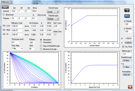
Figure 1‑2 A simple absorption and breakthrough plot

Here we have an elastomer with a medium-sized, linear solvent. At low concentrations the diffusion rate is 1E-07 and above 0.333 volume fraction the rate becomes constant at 3.8E-07. The solvent has a RED number of 0.94 and an estimated surface concentration of 0.24. After 2.1min it has broken through (at a 0.1% level) to the other side of a 0.2mm sample. Shortly after that, the concentration gradient stabilizes to its final form with the absorption being balanced by the desorption. The “Square Root” option has been chosen which creates a straight-line in the increase of % concentration.

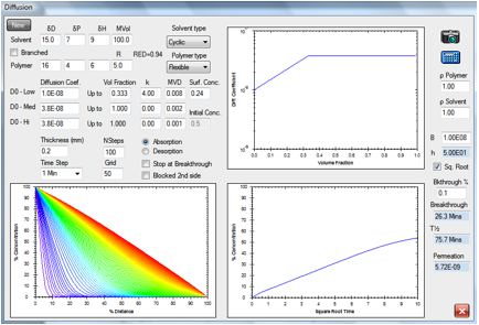
Figure 1‑3 The same absorption but with a slower-diffusing molecule

A cyclic molecule of the same HSP with twice the molar volume is estimated to have a diffusion rate a factor of 10 slower, so breakthrough time is 26.3min.

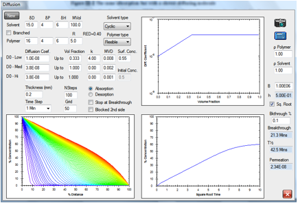
Figure 1‑4 A slower-moving molecule but a lower RED number

A solvent with a RED number of 0.4 but the same cyclic structure and molar volume is estimated to breakthrough in 21.3min simply because the surface concentration is estimated to be higher at 0.55.

Desorption

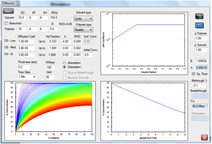
Figure 1‑5 A classic desorption curve

The same solvent is assumed to have saturated the block of polymer and is now allowed to desorb via the left-hand surface (the right-hand being assumed to be blocked). The coloured curves show the solvent distribution with time, the red curve being the distribution after 100min.

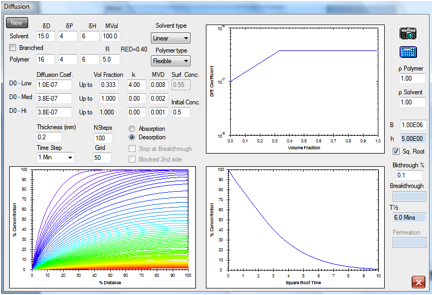
Figure 1‑6 Desorption by a smaller, faster molecule

The linear molecule, 100 molar volume, desorbs considerably faster.

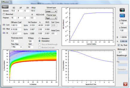
Figure 1‑7 Same molecule but desorption from a rigid polymer

This behavior resembles the formation and drying of a polymer film from solution. Such behavior has been studied in detail by Hansen in Hansen, C.M., A Mathematical Description of Film Drying by Solvent Evaporation, J. Oil Colour Chemists’ Assn., 51, No. 1, 27-43 (1968) and in the Doctoral thesis from 1967 that is available as a PDF file on www.hansen-solubility.com by clicking on the cover page.

In a crystalline polymer, the shape is highly skewed. Because the diffusion rates are relatively high through the bulk, the profile is rather flat. At the edge, where concentration is very low, the diffusion rate plummets.

“Surface resistance”

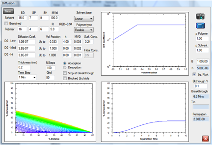
Figure 1‑8  “Surface resistance” coming from a Mass Transfer limitation in a permeation study

In this permeation example, the “surface resistance” comes because the “B” value (ratio of diffusivity to surface resistance) has become significant at the entry surface. When there is a significant surface condition at the entry surface, where there is (usually) contact with a liquid there can also be a significant surface condition at the exit surface, where the contact is with a gas. This possible effect at the second surface is not considered in the present discussion. The diffusion and surface effects are finely balanced. Solutions to the diffusion equation for absorption, as modelled here in Figure 14-8 and in Figure 14.9, give the so-called “s-shaped” or “sigmoidal” absorption curve. This behaviour is often misinterpreted in the literature as being anomalous diffusion since the absorption is not a straight line versus the square root of time, which is called “Fickian”. The other forms of “anomalous” diffusion that are incorrectly interpreted in the literature have the coined terminology Case II and Super Case II. These are discussed in the following. An article in the European Polymer Journal (Hansen, C. M., The significance of the surface condition in solutions to the diffusion equation: Explaining “anomalous” sigmoidal, Case II, and Super Case II absorption behaviour, European Polymer Journal 46 (2010) 651–662) explains these so-called anomalies with the following abstract:

“Absorption into polymers is frequently described by the terms Fickian, sigmoidal (S-shaped), Case II, or Super Case II. This terminology is used to describe absorption that is respectively, linear with the square root of time, has a slight delay or S-shape with the square root of time, is linear with linear time, or increases more rapidly than with linear time. Solutions to the diffusion equation, Fick’s second law, that include a potentially signficant surface condition are shown to reproduce all of these. Sigmoidal absorption results when the surface condition is moderately significant for either a constant diffusion coefficient or exponential diffusion coefficients. Exponential diffusion coefficients and a lower surface mass transfer coefficient result in Case II type behavior, with Super Case II behavior resulting when the surface condition becomes still more significant. The results reported here are supported by extensive experimental data with reasonable and verifiable values for the diffusion coefficients and surface mass transfer coefficients.”

The following figures show these effects for absorption.   

               

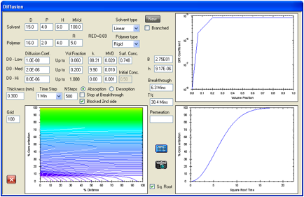
Figure 1‑9 Simulation of water absorption into untreated PVA films (Sigmoidal Absorption).

The S-curvature in the lower right figure matches the experimental data in [Hasimi, A., Stavropoulou K.G., Papadokostaki M, Sanopoulou M. Transport of water in polyvinyl alcohol films: Effect of thermal treatment and chemical crosslinking. European Polymer Journal Vol. 44, 4098-107 (2008)] very well. The initial curvature is very dependent on the concentration dependent diffusion coefficients used, so improved diffusion coefficient data, especially at low concentrations may remove any minor differences. The concentration dependent diffusion coefficients that were used are given in the upper right corner of the figure. The concentration profiles as a function of time confirm that there is diffusion resistance of significance only up to concentrations near 0.1volume fraction or less. At higher concentrations diffusion within the film is much faster than water can get to and through the exposed surface. The experiments are primarily a measure of a mass transfer coefficient of unknown origin (test setup, surface effects, etc.) as reported in (Hansen 2010) cited above.

 

Case II absorption

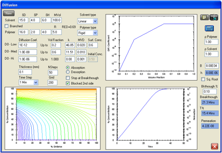
Figure 1‑10  Simulation of Case II type absorption

The straight line absorption curve at the lower right is typical of Case II absorption. The h value, 8(10)^-6 cm/s, is reasonable as is the diffusion coefficient profile reported in Figure 14-1. The tail at greater than 90% absorption would be reduced for higher h values, which could also be reasonable. This kind of tail can be seen in the literature for the polystyrene/n-hexane system in an often cited reference for Case II behaviour [Jacques, C.H.M., Hopfenberg, H.B., Stannet, V. in Permeability of Plastic Films and Coatings. Hopfenberg, H.B. Ed. New York:Plenum Press;1974, p.73.]. An initial curvature upward is also possible with an increased h value.

Super Case II absorption

As we’ve stressed, there is no need to invoke any new principles to explain exotic behaviours such as Super Case II. To make it appear, we simply have (a) a large dependence of diffusion rate on concentration as in Figure 14-1, which means a very low D₀, and (b) a significant surface entry resistance. Here’s a specific example:

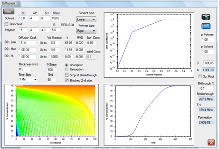
 Figure 1‑11  Simulation of Super Case II absorption

A significant surface condition coupled with the measured concentration dependent diffusion coefficients given in Figure 14-1 above leads to a marked increase in absorption rate well after the absorption process has started. There is an exponential approach to the equilibrium value at the very end of the absorption process because the driving force for further absorption at the surface has become small. The significant surface condition in such cases can probably be attributed to the hindered entry resistance, perhaps like a skin, described below since the value of h is only 1(10)^-7 cm/s, but some combination with one or more additional sources of significant surface condition resistance is also possible.

Significant surface condition caused by hindered entry

The expected phenomena that hinder mass transfer in absorption will also be capable of hindering mass transfer in desorption, with the opposite sign in the mathematics, of course. These include diffusion through a stagnant gas layer, heat transfer to or from the given surface, wind velocity, etc. In addition to these easily recognized effects a more subtle cause of a significant surface condition has been elucidated recently [Nielsen, T. B. and Hansen, C. M. Significance of surface resistance in absorption by polymers. Ind Eng Chem Res, Vol.44, No.11, 3959-65 (2005), and also in the Handbook]. This is an entry or hindered surface passage resistance dependent on the size and shape of the entering molecule, and, of course, the polymer surface morphology. For smaller molecules such as tetrahydrofuran, n-hexane, and 1,3-dioxolane there is no significant surface condition effect of this kind for absorption into the COC polymer Topas^? 6013 from Ticona. With more extensive absorption experiments it was obvious that entry into the polymer was more difficult as the size of an absorbing molecule increased or its structure became more complicated, such as with side groups or cyclic entities. So-called S-shaped absorption curves, of the type shown above, with a pseudo time-lag were observed in a number of cases, including absorption of ethylene dichloride, diethyl ether and n-propyl amine. Solvents containing benzene rings and more complicated structures, such as acetophenone, phenyl acetate, 1,4-dioxane, and methyl isobutyl ketone are completely prevented from absorbing into this same polymer, in spite of HSP similarity to those that do absorb. This comparison indicates that they should readily absorb into the polymer. Their absorption after prolonged liquid exposures has been so little that it could not be detected. In such cases there is no significant transport resistance in the external media, so it has been postulated that there can also be a significant surface condition caused by an entry or surface passage resistance. This type of resistance deserves much more attention to fully understand what is happening. One can surmise however, that for most polymers there will be smaller molecules that enter readily, and very large molecules (such as a polymer molecule of the same kind) that will not be able to enter at all. Between these extremes there will somewhere be a range of molecular sizes and shapes where entry is possible but becomes retarded since the molecules cannot rapidly find suitable sites to absorb even though they may be adsorbed. The orientation of adsorbed molecules at such selected sites where absorption is possible is thought to be a key element in this type of resistance to transport. Thermal treatments can be expected to affect surface morphology, such as in known from rapid cooling in injection molding. Because of this, thermal treatments having an effect on surface morphology may also be a factor in this behaviour.

Permeation

The modeller automatically calculates permeation rates in g/cm²/s. This is of necessity an approximation depending on how long you run your simulation – the value displayed gradually asymptotes to the final value as the system equilibrates.

For those who prefer a plot of  the integrated  amount permeated that option is available in the 3^rd Edition, along with an extrapolation down the straight part of the curve to estimate the “lag time”. Such plots are common in, for example, the skin permeation literature. Numerous examples of permeation in chemical protective gloves are given in Chapter 17.

Summary

With this powerful modeller you can explore a wide range of systems, including the important “Breakthrough” type of experiments where both kinetic and thermodynamic (HSP) factors play a role. Examples of Fickian and what is commonly and erroneously called non-Fickian or anomalous diffusion have been given to help guide your efforts.

The next two chapters treat diffusion in protective gloves in more detail, showing how improved judgment of glove safety is possible and how one can actually deduce the concentration dependent diffusion coefficients from permeation data.

 

E-Book contents | HSP User's Forum