Chapter 21, Cleaning by numbers (HSP for Surfactants)

         

This chapter is co-authored by Dr Richard Valpey III of SC Johnson. We are grateful to Richard for his expert technical input and to his company, SC Johnson, for giving us permission to use their surfactant HSP data. Responsibility for errors in this chapter remains with Abbott as per his guarantee.

The good thing about surfactants is that there are so many to choose from. The bad thing about them is the same – that there are so many to choose from. Many would-be users of surfactants despair at having to sort through so many different surfactants in search for the perfect one.

The search is helped somewhat by well-known numbers attached to surfactants such as HLB (Hydrophilic- Lipophilic Balance), Aniline point, KB (Kauri Butanol) value. But these provide surprisingly little scientific insight into a specific surfactant.

HLB was originally determined by a time consuming determination of emulsion stability. Griffin measured the stability of two types of emulsions (oil-in-water and oil-out) formed by a series of oils in the presence of surfactants. He then fit the results to a systematic ranking and called it the hydrophile lipophyle balance (HLB). It is time consuming because approximately 75 emulsions were made for each HLB determination.

Becher suggested that HLB relates to free energy according to the following equation

Where:  and  are the free energy of micellisation associated with the lipophilic and hydrophilic moieties. C1 and C2 are scaling factors.

In its original form, HLB was a relative effectivity index, ranging from 0 to 40. Griffin acknowledged its limitation to nonionic surfactants.

Davies proposed eliminating this limitation by computing HLB based on the structure of the surfactant by assigning group numbers (GN) to various moieties according to the following equation:

The Davies method, which finds use in emulsion technology, produces negative HLB numbers, particularly when the lipophilic contribution is sufficiently large.

Despite difficulties in handling negative numbers and poor correlation to ionic surfactants, HLB is the most widely used tool for selecting surfactants.

In 1978, Little suggested a tool that overcomes these two difficulties. He proposed the following relationship between the Hildebrand Solubility Parameter δ and HLB. This method which was originally tested with nonionic and anionic surfactants, correlates poorly with cationic surfactants.

Given that HLB themselves frequently offer little insight to specific problems, and given that we know the limitations of the Hildebrand parameter, this correlation is not of much help.

Surely it makes sense to provide users with chemical insights into the functionality of the surfactants via HSP. There has been remarkably little work on this approach but by combining the earlier work of Beerbower with the recent work of Valpey we can make some progress.

The key fact is that we can think of surfactants as having 3 sets of HSP. The first is the hydrophobic portion. The second is the hydrophilic portion. And the third is the (weighted) average of the two just as with any mixture of solvents. The last is particularly important even if you don’t use it directly. Because it is a weighted average, it provides some of the insights from an HLB. So important is this weighting that we’ve added it to the software so it’s easy to do.

Here is a list of surfactant HSP partitioned in the above manner:

Surfactant	δD	δP	δH
SLES hydrophobe	16.0	0	0
SLES hydrophile	20.0	20.0	20.0
SLES Average	16.7	8.1	8.1
APG hydrophobe	15.5	0	0
APG hydropile	23.4	18.4	20.8
APG average	18.8	7.6	8.6
Span 80 hydrophobe	16.1	3.8	3.7
Span 80 hydrophile	18.1	12.0	34.0
Span 80 average	16.1	6.1	13.2
Alkyl sulfosuccinate hydrophobe	16.0	0	0
Alkyl sulfosuccinate hydrophile	20.0	17.0	9.7
Alkyl sulfosuccinate average	19.2	3.4	1.9
ST-15 hydrophobe	16.4	0.0	0.0
ST-15 hydrophile	16.2	7.8	10.4
ST-15 average	16.3	3.6	4.8

Table 1‑1 Estimated values for the three characteristic sets of HSP for typical surfactants. There is not yet experimental data to verify these estimates.

Let’s look more closely at Span 80 – Sorbitan oleate.

The “oleate” part can be imagined as methyl oleate with HSP of [16.2, 3.8, 4.5], or simply as [16, 0, 0] representing the pure hydrocarbon chain. We’ve chosen a group contribution method that gives the values shown below. The sorbitan can be calculated as [19, 13, 21] with a molar volume ~ 100.

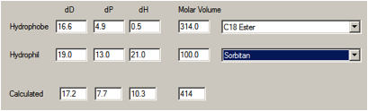
Figure 1‑1

The weighted average (calculated by summing the individual energies then dividing by the combined molar volume) is therefore biased towards the hydrophobic end – giving [17.2, 7.7, 10.3]. If Span 20 were considered, sorbitan monolaurate, then the individual HSP don’t change much, but the reduced molar volume of the laurate moiety (~215) shifts the average to [17.5, 9.2, 12.1].

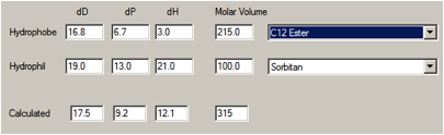
Figure 1‑2

No doubt you’re starting to see the problems with this approach. There are a few assumptions that have to be made. Where do you draw the line between hydrophobe and hydrophile? How do you estimate the HSP and molar volumes for the chunks into which you’ve divided the molecule?

We’ve attempted to answer some of those questions for you by providing our best estimates of many of the common groups used in surfactants. By selecting one of the hydrophobes and one of the hydrophiles (it’s up to you whether that combination can actually exist) you at least have a reasonable starting point for your own explorations. But our values are only for guidance, you should use your own judgement for your particular surfactants.

For the 3^rd Edition we’ve added an optional Y-MB calculation of the surfactant HSP. Wherever there are meaningful SMILES values for the head and tail and also meaningful Y-MB fragments available, the head and tails SMILES are stuck together into a single SMILES and sent to Y-MB.

At this stage in surfactant research we have no good data to give you. Instead we’ll go out on a limb and make some predictions. Let’s take 5 standard “soils” (see the Handbook for an explanation of these 5. The HSP numbers in the Handbook differ from those shown here)

No.	Soil	δD	δP	δH
1	ASTM Fuel “A”	14.3	0	0
2	Butyl Stearate	14.5	3.7	3.5
3	Castor Oil	15	6	8
4	Ethyl cinnamate	18.4	8.2	4.1
5	Tricresyl phosphate	19	12.3	4.5

 

Now let’s calculate the distance between each of these soils and 5 surfactants

Surfactant	1	2	3	4	5
SLES	14.5	10.6	8.4	2.8	2.6
APG	14.6	10.7	7.8	4.6	6.2
Span 80	15.0	10.5	5.6	10.4	12.2
Alkyl sulfosuccinate	10.5	9.5	10.7	5.5	9.3
ST-15	7.2	3.8	4.8	6.3	10.2

 

If you believe this approach to surfactants, then from the table you can instantly work out that each stain has an optimal surfactant. Stain 1 would best be removed by ST-15, though the distance is so large that it might not work at all. ST-15 will be also be best for stains 2 and 3, with more success, and SLES would be best for stains 4 and 5.

The “if” at the start of the previous paragraph is rather important. Classic thinking about surfactants tends to assume that the hydrophobic tail does the interaction with the soil and the hydrophilic head does the interaction with the water so that the tail + soil get swept away. There is an obvious problem with this classic thinking. The tails of most surfactants are remarkably similar and therefore the cleansing power should be fairly similar as long as the head is swept away in the water. The very large differences in cleaning power of different surfactants are therefore not naturally explicable using such simple ideas. The HSP model suggests an alternative approach to rational removal of soils.

Of course, the classic model includes the formation of micelles as the actual cleaning agents, and the different chains give different critical micelle concentrations and, therefore, different behaviour in the cleaning environment. Notions such as Critical Packing Parameter depend strongly on the relative size of head and tail. The simplistic HSP approach says nothing about this important element of surfactant behaviour. But of course the different chain lengths will also have different HSP and molar volumes, which, in turn, determine their solubility in water and, even more importantly, their relative solubility in the two phases and thus the delicate balance which appears as the PIT – Phase Inversion Temperature. Perhaps the most interesting aspects of HSP and surfactants will be their use in non-aqueous dispersions, where matching HSP of the surfactant ends to the HSP of the respective phases would seem to be a helpful exercise.

Nevertheless, we’re happy to predict that an intelligent use of HSP will prove highly insightful for many cleaning applications. We have some evidence from our own commercial activities that these predictions are indeed helpful. But despite the fact that this approach was first suggested by Beerbower many years ago, only recently has it been looked at with fresh eyes and more powerful ways of predicting HSP values. The Inverse Gas Chromatography (IGC) technique discussed in the Chromatography chapter gives hope that the HSP of numerous surfactants will be measured experimentally, which will be an important addition to our knowledge base. We are confident that we will be hearing more about coming clean with HSP.

Update for the 4^th Edition

The big advance in surfactant theory has come from the HLD theory of Salager as extended by Acosta to form HLD-NAC. This simple, numerical approach offers great power and puts to shame naïve ideas of HLB and invalidates many of the formulation ideas behind CPP (Critical Packing Parameters). This eBook is not the place to discuss HLD-NAC. The free software and apps provided at www.stevenabbott.co.uk/HLD-NAC gives formulators a quick way to learn how to apply the theory.

But HLD-NAC requires knowledge of the “oil” with which one is formulating. In particular it requires the Equivalent Alkane Carbon Number (EACN) for the oil. HSPiP can now estimate the EACN from a SMILES input. The estimation is only as good as the dataset used to model it. There is an unfortunate lack of reliable EACN values across a wide range of molecules. As HLD-NAC becomes more used and EACN values for more oils are measured the estimation scheme will become steadily more reliable.

 

E-Book contents | HSP User's Forum