Chapter 22,　Chromatography – HSP creator and user (Retention Times and HSP) 

Chromatography is about controlled interactions between chemicals in one phase and those in another. It is therefore not surprising that HSP can play an important role in understanding the outcomes of a chromatographic process.

One important aspect of chromatography is as a creator of reliable HSP. Given how hard it can be to get HSP for chemicals and polymers, it’s good to know that those with the right chromatographic kit can determine HSP relatively easily.

HSP can also be used to explain and, more importantly, predict retention times in some chromatographic processes. So chromatography can be both a creator and user of HSP.

Creating HSP with chromatography

The archetypal method is Inverse-phase Gas Chromatography (IGC) where the solid phase is made from the polymer to be investigated and the retention times are measured for a series of solvents with known HSP. The closer in HSP the solvent is to the solid phase, the more the solvent will tend to linger within the solid phase, so the retention time will be higher. However, as we will see, IGC also depends on other factors such as vapour pressure.

The key issue is how to extract HSP from the retention data. The first step is to convert the retention times into specific retention volumes Vg. These can then be converted into Chi parameters. Finally, the HSP can be found by doing a linear regression fit to the formula relating Chi to HSP. The papers of Professor Jan-Chan Huang’s group at U. Massachusetts-Lowell are good examples of this, J-C Huang, K-T Lin, R. D. Deanin, Three-Dimensional Solubility Parameters of Poly(ε-Caprolactone), Journal of Applied Polymer Science, 100, 2002–2009, 2006. Their data can be recast into a format that uses the standard HSP distance (in this case, distance-squared). The famous factor of 4 is automatically included. Careful analysis by Professor Huang’s group found that by having no factor of 4 the errors were rather large and they included a factor as a fitting variable. Its optimum values varied from 2.6 to 4. The group were very much aware of the theoretical value of 4 but postulate that at the higher temperatures of these experiments the lower values may be justified.

Here is the fit for their data on polycaprolactone, using the revised version of their approach

Equ. 1‑1 Chi = C1 + MVol *C2 * (4 * (δD_p-δD_s)² + (δP_p-δP_s)² + (δH_p-δH_s)²)

Where constants C1, C2 and the Polymer HSP (δD_p, δP_p, δH_p) were the fitting parameters.

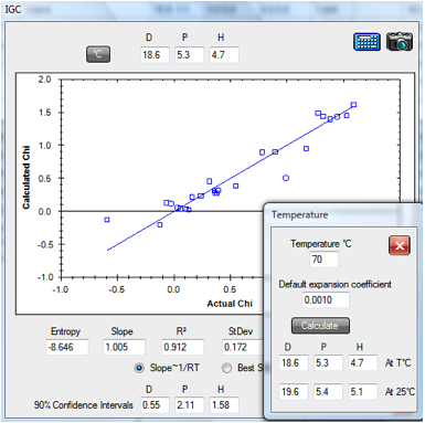
1‑1 IGC fit of polycaprolactone data

From this fit, the values [18.6, 5.3, 4.7] are close to Huang’s optimized fit (using 3.2 instead of the factor of 4) of [18.5, 4.2, 5.6]. The fitting program contains extra information based on Huang’s analysis. An Entropy value captures the size of the RTη term (using an approximation of 100 for the Molar Volume of the stationary phase). And a 90% Confidence Interval is estimated for δD, δP and δH using an approximation to the method described in Huang’s paper.

The program offers a choice of fits to give the user some idea of the robustness of the results. The “C2*RT ~1” option forces C2 to be close to its theoretical value of 1/RT. Alternatively you can optimize to the minimum Standard Deviation. You can also explore the robustness of the fit manually be entering your own values into the δD, δP and δH fields.

Note that the Temperature (°C) option is used so that solvent HSP are calculated at the 70°C of the dataset as discussed below. When translated back to 25ºC the values become [19.6, 5.4, 5.1].

The dataset used (Polycaprolactone Huang Probes.hsd) is provided with HSPiP along with a fuller dataset (Polycaprolaction.hsd) which gives a fit of [19.4, 5.5, 5.6].

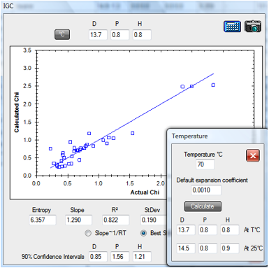
Similarly the 70ºC PDMS data set (PDMS.hsd) gives a room temperature value of [14.5, 0.8, 0.9].

 

Figure 1‑2 IGC fit of PDMS data

Huang’s analysis is of data from M. Tian and P. Munk, Characterization of Polymer-Solvent Interactions and Their Temperature Dependence Using Inverse Gas Chromatography, J. Chem. Eng. Data 39, 742-755, 1994. HSD files for all the polymers in this paper are included with the HSPiP as a contribution to the use of IGC for HSP purposes. Note that the Chi parameters are calculated in the Tian and Munk paper. See below for doing your own Chi calculations.

If that were all there is to it then everyone would be using IGC to measure HSP of their polymers. One issue is that IGC has to take place at a temperature where the polymer is suitably “liquid”. In the example above, the HSP for the polymer are those at 70ºC. The fitting procedure compares the polymer HSP with the solvent HSP. But of course, the validity of the calculation depends on having good values for the HSP of the solvents at these elevated temperatures. The standard approximation for calculating HSP at different temperatures comes from Hansen and Beerbower:

Equ. 1‑2 d/dT δD = -1.25a δD

Equ. 1‑3 d/dT δP = - a δP/2

Equ. 1‑4 d/dT δH = -(1.22 x 10^-3 + a/2)δH

a is the thermal expansion coefficient. For the IGC technique to become more popular we need ready access to reliable calculations of HSP at different temperatures for the common solvents so that data from different IGC users will be comparable. HSPiP includes those calculations based, wherever possible, on known temperature dependent as. The full Sphere Solvent Data set contains the appropriate coefficients for calculating a at a given temperature from the constants a, m and T_c (the critical temperature):

Equ. 1‑5 a = a*(1-T/T_c)^m

Note that this equation is only valid over a defined temperature range. For solvents with no constants or outside their valid range, HSPiP uses a user defined default value for a.

However, many molecules which are adequately “liquid” at room temperature can be used as the “solid” phase for IGC. The paper by K. Adamskaa,, R. Bellinghausen, A. Voelkel, New procedure for the determination of Hansen solubility parameters by means of inverse gas chromatography, J. Chromatography A, 1195, 2008, 146–149 measures the HSP of a group of excipients: Cetiol B, Lauroglycol FFC, Labrasol, Miglycol and Tween 80. They used a similar fitting procedure for deriving the HSP. Professor Voelkel kindly sent the Chi data for Tween 80 and here is an Excel fit of their data:

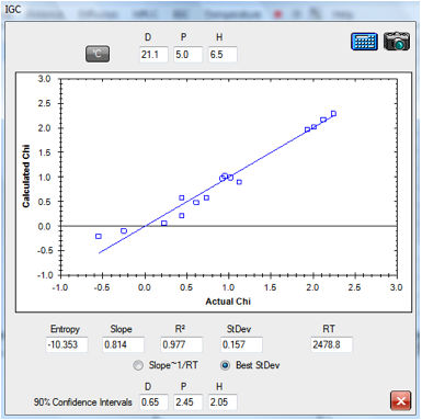
1‑3 IGC fit of Tween 80 data

 

The fitted HSP for Tween 80 [21.1, 5, 6.5] gives a suspiciously high δD value – for reasons that are unclear at this early stage of the science of interpreting these data.

The other issue is that the calculation of Chi from Vg requires knowledge of the partial pressure of each solvent at that temperature plus the second virial coefficient. This is an important point. If we measured the retention time of a new solvent on a range of IGC columns, we could do exactly the same calculation to determine the HSP of that solvent. But how many of us know the partial pressure and second virial coefficients of our new solvents?

As an aid to the IGC community, and as an attempt to provide a common standard for these tricky calculations, a calculator for converting specific retention volumes, Vg, to Chi parameters is provided. A representative range of solvents is provided, spanning a good range of HSP space. For each solvent Tc, Pc and Vc (the three Critical Parameters) and Antoine A, B, C parameters are provided. These in turn are used to calculate P₀ (the saturated vapour pressure) of the probe solvent and B₁₁, the Second Virial Coefficient. It turns out that there are a number of alternative methods for estimating B₁₁ from the Critical Parameters, and they give different results. Happily, the exact value of B₁₁ is not hugely important so we don’t have to worry too much. To help users, two representative methods are used. The first has been popularised by Voelkel and uses Tc and Vc. The second is coded BNL after Blu, Nesterov and Lipatov, which uses Tc and Pc. In general the BNL method gives larger (more negative) B₁₁ values than the Voelkel method. The program shows you the B₁₁ values (and P₀) so you can see for yourself. You can find out all about these methods (and others) from A. Voelkel,, J. Fall, Influence of prediction method of the second virial coefficient on inverse gas chromatographic parameters, Journal of Chromatography A, 721, 139-145, 1995. The only other inputs are the density of your test material and its “molar volume”. Both values are controversial. The density, of course, changes with temperature. But as the molar volume of the solvents also change with temperature (and are not explicitly calculated) the assumption is made that the relatively small density effects cancel out. The “molar volume” is often an estimate – what, for example, is the molar volume of a polymer? The recommended guess is to put in the molecular weight of a typical monomer unit. Errors in this parameter mostly result in an offset of the calculated Chi values rather than a significant change in their relative values. The calculation of HSP is relatively insensitive to this offset. Because you can instantly see the effects of varying the density and the “molar volume” you can make your own judgement of how valid the calculated HSP really are. It’s important to note that these sorts of judgements about B11, density and molar volumes are generally not explored in IGC papers. By making them explicit, and by encouraging the use of the same basic dataset, we hope that the IGC community will start to standardise on one approach so that calculated HSP are relatively more meaningful.

So although IGC has considerable promise for determining HSP of polymers  and looks excellent for intermediate molecules such as excipients, oligomers and surfactants at room temperature, its use for taking a set of known stationary phases and deducing HSP of solvents looks like something that is not for the faint-hearted.

There’s one key point about IGC. It’s relatively easy to get good fits from just about any data set. But the value of that fit is questionable unless the test solvents cover a wide region of HSP space. This is the same issue as other HSP fitting. Having lots of data points in one small region is far less valuable than having the same number of data points spread out over the full HSP space. One IGC paper used 5 similar alkanes, 2 similar aromatics, 3 chlorinated hydrocarbons and one simple ester. This is a very small portion of HSP space! So if you want really good IGC data make sure you challenge the material with solvents from the full range of alkanes, aromatics, ketones, alcohols, esters, amines etc. etc. The wider the range, the more likely it will be that your calculated HSP are meaningful. That’s why in the Vg to Chi calculator we’ve included not only solvents typically found in IGC papers but a few more that will help cover a broader HSP range. By providing a consistent set of Antoine and Critical Parameter values we will have saved IGC users a lot of work!

GC prediction via GCRI – Gas Chromatography Retention Index

It would be very useful if we could predict in advance the exact retention time of a chemical on a GC column. But of course this is not directly possible as retention time depends on numerous specific variables in the GC analysis: column type, column dimensions, temperatures, flow rates etc.

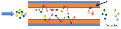
A useful substitute is the GCRI. We know that the retention time of straight chain alkanes form an orderly progression from CH4 to C2H6 to C3H8 … And if we give each of these alkanes a retention index = 100 x number-of-carbon-atoms we can say, for example, that if a chemical elutes at precisely the same time as heptane then its GCRI is 700.

If the chemical elutes somewhere between hexane and heptane then, by definition, the GCRI is somewhere between 600 and 700. Kovats proposed a formula for calculating the GCRI. Suppose the lower n-alkane elutes at time A, the higher (n+1)-alkane elutes at time B and the chemical elutes at a time X between A and B then:

Equ. 1‑6 GCRI = 100 * ( log(X)-log(A))/(log(B)-log(A)) + n * 100

If, in the example above, hexane eluted at 60 seconds, heptane at 80 seconds and the chemical at 70 seconds then GCRI = 100 * (1.845-1.778)/( 1.903 - 1.778) + 600 = 654

If we can predict GCRI from the chemical structure then we can provide an accurate estimate of the retention time in a specific column provided we know the retention times of the alkane series.

The simplest way to estimate GCRI is to say it depends only on the boiling point of the chemical. This turns out to be an impressively good predictor. The reason for this is simple – at the very low concentrations of the chemicals in the GC the behaviour of the gases is close to “ideal” so molecules hop on and off the support more or less according to their volatility.

 

 

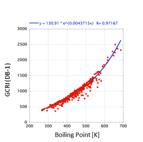
But “impressively good” isn’t “good enough”. In the figure for GCRI values on a DB1 (Polysiloxane) support the general trend with boiling point is clear, but when you look more closely at the graph you see that for a given boiling point the GCRI can vary by 200-300 – much too large an error to be a useful predictive tool.

Clearly the assumption that the chemical is behaving in an “ideal” manner is not working. And of course we know that different chemicals will interact more or less strongly with the support phase. And a good measure of that interaction is the HSP distance.

It then seemed obvious to add a correction term that depended on the classic HSP distance calculation involving δD, δP and δH and the values for the chemical, c, and support s. When this was tried, the results were worse than using just the boiling point! What had gone wrong? One hypothesis is that the δD value is already “included” in the boiling point (for example, Hildebrand and Scott have shown that for simple alkanes, δD ²=RT+17.0*Tb +  0.009*Tb²⁾. If the δD term is removed from the distance calculation so that:

Equ. 1‑7 Distance² = (δPc-δPs) ² + (δHc-δHs) ²

then the fit becomes excellent:

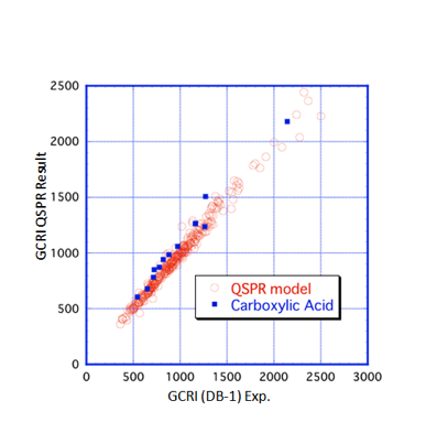
The correlation formula used (via a Quantitative Structure Property Relationship model) is:

Equ. 1‑8 GCRI = -220.27+209.51*(BPt*0.000519+1)^8.52* (DistPH*-0.0372+1)^0.156

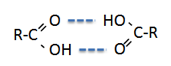
Well, it’s almost excellent. The main exceptions are the carboxylic acids, shown in blue. Perhaps this is because the acids tend to form dimers:

 

 

We’d like to claim that we have a universal formula for GCRI. However, the only other extensive dataset available to us, using the DX1 column, has a slightly different fitting formula which also requires the MVol. We would need more datasets before being able to resolve this dilemma. So the GCRI modeller lets you choose between these two (quite similar) columns. If you try other values for the HSP of the columns we can’t say what  your predicted results will be like. If you have access to other GCRI datasets for other columns, we’d be delighted to fit them and try to get a more generalised rule.

In the HSPiP software we implement the correlation via the Y-MB functional group method using neural network fits for the boiling point and the HSP, though manual entry of the values is also possible if they are known independently.

 

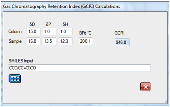
In this example the GCRI for a branched aldehyde/alcohol is calculated as 947. If you wanted to test the purity of this compound in a GC column you would simply set up conditions that gave you reasonable elution times for nonane and decane and you would find your compound nicely resolved. If you thought that your sample would have impurities with one less and one more carbon in the main chain then the GCRI values for these two molecules are quickly calculated as 845 and 1034 respectively so you would set up your GC column for conditions where octane to decane (or undecane) eluted in reasonable times. If you found a peak at around 1149 some simple experimentation with likely contaminants show that it is likely to be the dialcohol:

 

 

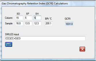
If you wanted to explore the effect of changing to a support with different HSP values then it is simple to find that, for example, that the original molecule will move from 947 to 1031 for a slightly more polar column. Changes in the δD value make, of course, no difference to the calculated GCRI.

 

 

HSPiP, therefore, provides you with a very powerful predictive tool for your GC work.

 

HPLC

There are good theoretical reasons for believing that High Performance Liquid Chromatography (HPLC) should conform exactly to HSP for systems other than those that depend on ionized (acid/base) or size-related separation. The principle is simple: the analyte has to “choose” between residing in the stationary phase of the column and the mobile phase of the eluent. And the “choice” is a simple HSP calculation. The parameter of interest is k’, or “capacity factor” (which is calculated from the retention time and the column volume, so a large k’ represents a large relative retention time), and the key formula is:

Equ. 1‑9 ln k’ = C1 + C2 * MVol * (Distance_ma – Distance_sa)

where C1 and C2 are constants, m=mobile phase, s=stationary phase and a=analyte, MVol is the molar volume of the analyte and the distances are the classic square distances:

Equ. 1‑10 Distance²_ma = 4*(δD_m-δD_a)² + (δP_m-δP_a)² + (δH_m-δH_a)²

Equ. 1‑11 Distance²_sa = 4*(δD_s-δD_a)² + (δP_s-δP_a)² + (δH_s-δH_a)²

What is surprising is that these simple formulae have been used very little. Why is this? Sadly, the pioneering papers were written on the basis of rudimentary Hildebrand solubility parameters. As we now know, without the partitioning into D, P and H, the resulting correlations simply aren’t reliable enough and the technique of correlating with solubility parameter quickly fell into disrepute. Later attempts failed because reliable values of HSP were hard to find and relatively small errors in HSP lead to large errors in the predicted k’. For example, Ethyl benzene and Methyl benzene (Toluene) are very close in HSP space and if we were interested in them as solvents we would not be too bothered if a parameter were out by 1 unit. But for HPLC, Ethyl benzene and Toluene are classic test analytes which separate readily and although the MVol surely has the most significant effect (123/107), a small error in the HSP can rapidly be amplified by the squared effect in the two distance calculations.

An excellent data set covering a good range of analytes, columns and solvent mixes comes from Professor Szepesy’s group at the Technical University of Budapest. The group have explicitly rejected solubility parameters because they were not of sufficient predictive value.

It was a good test to use the most recent HSP data set to see if it could do a good job in fitting the data. This is a tough challenge as there is a lot of high-quality retention data to be fitted using pure thermodynamics with no adjustable parameters. At the start of the fitting process the key unknowns are the HSP of the column materials and the HSP of the eluent. The prime data set uses 30/70 acetonitrile/water and it was straightforward to confirm that by using the 30/70 mixture of the standard acetonitrile and water values there was an adequate fit. The data could then be processed to find that [15, 0, 1] provided an adequate fit for the first stationary phase tried – reasonable for a classic C18 column. Other columns in the data set surprisingly gave [15, 0, 1] as about the best fit, including one –CN column that is supposed to be more polar. The differences in k’ values between the columns depended strongly on the Slope factor (C2). The variation from column to column made no obvious sense to us till the correlation was found with the %C values (% Carbon) provided for each column in the data set. Large %C’s gave large slopes (and therefore large separations).

The challenge now got tougher given that the fits had to work not only for one solvent blend but for a range. This was initially unsuccessful. The changes in k’ values were larger than the change in the HSP of the solvent blend would naturally produce. The literature provided various suggested fixes for this much-observed phenomenon but nothing simple and elegant suggested itself. The other problem was that the basic theory said that the Slope value should be a constant, equal to 1/RT whereas it depended on the column and was a factor ~25 smaller than 1/RT.

In the end a simple solution emerged that gave adequate data fits across 60 data sets: 5 columns, two different solvents (acetonitrile, methanol) and 6 solvent ranges (20, 30, 40, 50, 60, 70% solvent). The Slope term was modified to C2 * (1-0.013 * % Solvent). So far there is no theoretical explanation for this fudge factor nor for the fact that C2 is out by a factor of ~25, but the fit to a large number of totally independent data sets seems to be compelling evidence that the approach has many merits.

Having now fitted many 10’s of data sets with a considerable degree of success, we need to point out that HPLC systems do not operate in the sort of HSP zone to which we are all accustomed. The reason for this is explained in a groundbreaking paper on using solubility parameters (alas, ahead of its time) by Schoenmakers’ team in Chromatographia 15, 205-214, 1982. They show that the stationary and mobile phases are very far apart in HSP space. This amplifies the separation and (therefore) selectivity. What follows from this is that the HSP of the stationary phase have a surprisingly small effect on the separation. Changes in the mobile phase have a significant effect, but even this is modest when you consider the vast change in HSP between, say, 100% acetonitrile and 100% water. The clever thing about HPLC is that the only thing which makes a big difference to retention time is the molar volume and HSP of the analyte. It’s worth repeating that the modest effect of mobile and stationary phase and large effect of HSP falls very naturally from Schoenmakers’ analysis.

What’s not so obvious is the very significant effect from molar volume. The large separation between toluene and ethyl benzene or between the various parabens also included in the Szepesy data set comes almost entirely from the molar volume effect. One obvious explanation for this is some sort of diffusion limited or size-exclusion effect. But that’s not what the basic theory says. The molar volume term comes in simply because the thermodynamics say that interaction energies are HSP/Molar_Volume. This large effect and its scientific explanation are a particularly satisfying vindication for the HSP approach.

Here are two plots that show the reasonable degree of success of the technique. The data are for columns at either end of the spectrum. The first is a classic hydrophobic C18 column and the second is a classic polar CN column. The results are based on an optimum HSP of [15, 0, 1 ] value for both stationary phases as discussed above. For the CN column the retention times are rather small, particularly for the left-hand side of the graph. In the original paper, the authors discarded the data points for Caffeine and Hydroquinone because their retention times were too small. In each case the plots are of actual v predicted ln k’. Below the plot of the fit is an indication of what the idealised HPLC trace would look like with the fitted values. The value of this will emerge in a moment:

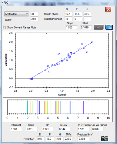
Figure 1‑4 A reasonable correlation for the C18 column:[15, 0, 1]

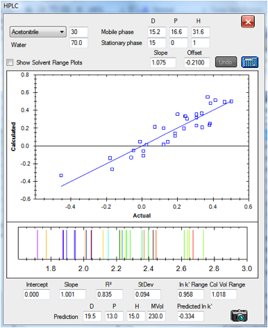
Figure 1‑5 The correlation for the CN column: [15, 0, 1] It’s noisier partly because it spans only a small range of column volumes. The data set is slightly different from the one above, reflecting slightly different experimental protocols in the original papers

The software allows you to interact freely with the data. You can create mobile phase parameters directly by choosing the solvent (Acetonitrile, Methanol or THF) and the relative percent with water – or you can directly enter your own values. The Calculator button automatically finds a slope/offset combination that give you a slope of 1 for the best fit line. You can alter these values manually if you wish.

The output includes the plot itself (moving the mouse above a data point reveals the solvent, actual and calculated data) then the intercept, slope, R² (goodness of fit) Standard Deviation and then the range over which the separation works in terms of k’ and in terms of column volumes. You can see that the –CN column fits all the chemicals in a range of 1-2.018 column volumes whereas the C18 covers 1-7.076 column volumes – giving you a choice of speed versus resolution.

The same C18 column run with 60% acetonitrile gives a relatively good fit. No fitting parameters were changed compared to the 30% values:

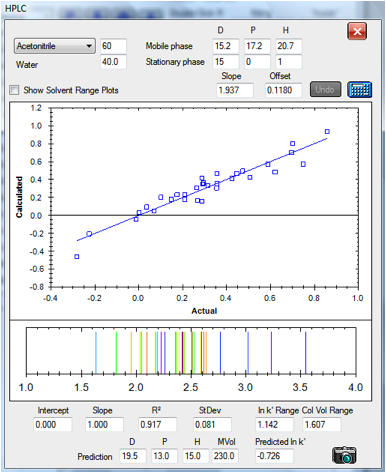
Figure 1‑6 The correlation for the C18 column at 60/40 acetonitrile/water

The fact that the same fitting parameters work for a large shift in the solvent blend indicates the power of the technique.

You can play live with these data yourself (plus the other HPLC data we have provided) and reach your own conclusion. One thing that playing “live” means is that you can alter the individual HSP from the standard HSPiP main form and see the effect on the HSP fit. We did this ourselves. The first was to fit p-Nitrophenol. It was obvious on the plot that the fit was very poor and we played with the values till the fit seemed reasonable. Only then did we realise that the published value for p-Nitrophenol was, regrettably wrong; the δP of 20.9 simply makes no sense. The second was to play with Caffeine - the point nearest the 1 column volume elution point and therefore the least accurate. The official value is an estimate. Perhaps the HPLC data are telling us to revise that estimate. The final adjustment was to Pyridine. The published value was re-checked and makes good sense, but was way off in the plots. When we looked at other examples of Pyridine in HPLC we noted that it was normally eluted as Pyridinium as the mobile phase is typically buffered to pH 3.0. Although the Szepesy data set was explicitly run unbuffered, we suspect that the value we have entered is for Pyridinium rather than Pyridine.

At this point the reader can go in two directions. The first is to say “They’ve fiddled the data to get the answer they wanted”. The response to that is that most “fiddling” with the data, although it could improve any single plot, generally made the plots over the full Szepesy data set positively worse. The second direction is to say “This looks like a powerful technique for understanding and predicting HPLC behaviour”. That’s why we’ve added the k’ range output (so users can think which column and/or solvent blend to use) and also the predictor. You can see in the screen shot how an analyte of [19.5, 13, 15] with a molar volume of 230 would behave in each of these columns.

The second direction makes sense. HSP and HPLC are a powerful combination – for predicting/understanding HPLC and for generating HSP values for use in other applications.

That’s also why the simulated elution plot has been included. When you change the % solvent (or the solvent itself) you can see how the eluted peaks are predicted to change. You can quickly see how two peaks close together can be separated or vice versa as you change the elution conditions. Similarly, if you click the Show Solvent Ranges you get a graphical idea of how the k’ of the individual analytes vary over the full 0-100% solvent range.

Expert HPLC users will object that the predictions of k’ are unlikely to be precise enough – they are, after all, predictions of ln k’, which can easily compress errors. This may well be true. But look at what the HSP approach offers. With one rather simple formula, with very few fitting parameters (and maybe after more investigation, no fitting parameters at all), a user or manufacturer can understand numerous fundamental aspects of what is going on in a separation. It seems, at the very least, that the HSP-HPLC approach should be investigated more deeply with alternative data sets.

Finally, here’s a data set prepared independently for us by Andrew Torrens-Burton, an expert Analytical Chemist at MacDermid Autotype. He gathered data for three different types of analyte, deliberately avoiding the aromatic test analytes used in the Szepesy data. The standard values for the C18 column calculated from the Szepesy data set were used for this analysis except that the slope is bigger – because this column happened to be twice the length of that used by Szepesy:

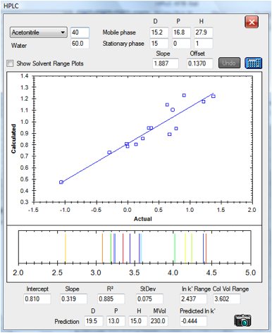
Figure 1‑7 The correlation for the set by Andrew Torrens-Burton

 

NMR Solvents

This is a very short section. We have not, so far, attempted any correlations between NMR and HSP, though it is clear that, for example, polymer-polymer interactions in solution will depend strongly on polymer-solvent interactions which can, in turn, be predicted via HSP.

But we see a very powerful use of simple HSP ideas to help the practical NMR spectroscopist.

One typical challenge is to find a solvent for carrying out NMR experiments for a given chemical. There are relatively few H-free solvents (i.e. deuterated chloroform, benzene etc. plus carbon tetrachloride) and if your chemical is not very soluble in any of them then you have problems.

But we know from HSP theory that a chemical can be insoluble in each of two solvents yet be soluble in a mixture, if that mixture is a good match for the HSP of the chemical.

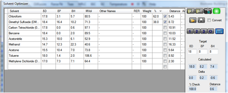
We’ve therefore provided a Solvent Optimizer dataset containing the most used H-free (deuterated) solvents.

If you enter the Target HSP of your chemical (perhaps estimated via Y-MB) and click the 2 button you instantly find a blend that gives you an optimum match. To be more precise you can click the 3 button to find a 3-solvent blend. If you are worried about cost you can even weight the solvents (high cost = low weight) so that the optimum blend uses less of the more expensive ones.

Armed with those data it is highly likely that you will find it much easier to get a higher concentration of your sample – at very little cost and very little trouble. In the following example a tricky [18 8 8] material is likely to be nicely soluble in the chloroform/DMSO mix – and it is highly unlikely that you would have tried that mix without help from the Solvent Optimizer.

 

 

E-Book contents | HSP User's Forum