Chapter 26, Exploring with HSP – (Generating and testing research hypotheses)

Many users of HSPiP have specific problems they want to solve: dispersing a particular nanoparticle, substituting a solvent for a particular polymer, finding an environmentally friendlier solvent blend, or perhaps something more exotic.

But HSP can also be used by the adventurous explorer to map out uncharted territory. All that’s needed is a bunch of HSP values, a vague hypothesis and some extra support software such as Excel.

Mission impossible – the insoluble polymer

Charles once had to find the best high-temperature solvent for a polymer that was insoluble in just about everything at room temperature. By chance it was known that one horribly toxic solvent could just about dissolve the polymer at ~150ºC – which was not a practical temperature. Knowing its HSP it was then possible to look for other solvents with HSP in that sort of region – just by sorting with RED number. This give a short list of possible candidates.

These were tested. Not surprisingly, given the single datapoint that started this process, about half the solvents were worse than the toxic one, but some were better. From this small dataset a better HSP estimate could be made and a few more solvents could be tested. This then gave a practical solvent that worked at ~120ºC.

That’s a simple example of exploration. The original hypothesis wasn’t brilliant. But it was a start. Without that hypothesis the solvent screening process would have involved many more experiments and much more time and expense. Now let’s look at some more complex explorations.

Screening with Distance maps

Suppose, (to take a specific example from the HSP user who inspired this chapter) you are interested in plant chemicals. You have an idea that solubility plays a key part (“a necessary but not sufficient condition”) in allowing a chemical to reach its target as, say, an anti-malarial. There are innumerable plant chemicals out there and if you don’t have access to a pharma-grade high-throughput screening system, how do you narrow down your choices?

The key is to have a method not of hitting winners (that’s asking too much) but excluding no-hopers. The problem with screening is that there are far too many possible candidate molecules, so anything which has a reasonable chance of excluding molecules that won’t work will be of great help.

Your starting point is a (small) list of chemicals that are known to work. If they have very different HSP then you need not bother to continue. But if (as is often the case) they are clustered near one region of HSP space then you can create a “target” value from this cluster (e.g. using a Sphere, taking an average, choosing your favourite), ready for calculating the distances from this target of the pre-screen molecules. An example of this approach has already been described in the DNA chapter with the cytotoxic chemicals.

So assemble your list of plant chemicals as a list of Names and SMILES and save it as a simple tab-separared .txt file – Excel does this for you no problem. Then find the File Convert option in Y-MB. If you have a lot of molecules and many of them are large you may want to go and have a cup of coffee while the computer does all the work. At the end of the process you have a .hsd file with estimated HSP values for most of the chemicals you presented. Most? It’s likely that any list of SMILES will have a few problem chemicals which Y-MB can’t handle. But if you drag the .hsd file into Excel it’s smart enough to recognise that it’s a tab-separated format dataset and you’ll get a nice table. Search for the word “error” using Excel and you’ll find the failed molecules. Simply delete their rows – you’ve got more than enough chemicals to screen in any case – or find the correct SMILES, convert them manually in Y-MB and Paste the values into Excel.

Now create a fresh line at the top which contains the target value which you think (or hypothesise) is a fair representation of the class. Then it’s easy to calculate the HSP distance of each molecule from your target D=sqrt(4*(δD_t-δD_i)² + (δP_t-δP_i)² + (δH_t-δH_i)²) where t=target and i=the i’th chemical. Excel can then sort by the distance column and you can decide a cut-off value for screening purposes – rejecting anything with a distance greater than that value.

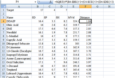
Figure 1‑1 A distance map in Excel, sorted to show the chemicals closest to the target

In this dummy example (of course there are more chemicals not included in the screen shot) I might decide that anything less than a distance of 4 is acceptable so would only test DDAIP to Octyl Salicylate.

If you want to be more sophisticated you can reason that anything with a MVol > 400 (or whatever value you choose) will be too slow to penetrate the target or too hydrophobic (see the chapter describing Ruelle’s solubility calculations) so you can do a sub-sort and remove those molecules that are too large. For this example I sub-sorted the <4 area by MVol, then resorted the area with MVol<300 to give my final shortlist:

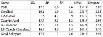
Figure 1‑2 A smaller list by excluding high MVol chemicals

If you’ve already got your list of pre-screening molecules in SMILES format then this whole exploration will have taken less than a few hours. What will you have achieved? At the very least, the molecules that pass your distance screen will be (because of their HSP match)  compatible with the formulation vehicle of your target active. If you’re an optimist then there’s also a good chance that these molecules will partition into the correct part of the cell or organism (because of the HSP match) and have a chance of working.

When we’ve tried such explorations we find them to be much more insightful than methods typically used in pharma: Lipinski’s Rule of 5 or LogP. No simple method will ever be perfect for identifying candidates but we believe that the HSP distance method has a lot going for it.

Finally, remember that there’s more to efficacy than solubility! It’s up to you to sub-screen the molecules for the right sort of chemical functionality. An example can be drawn from the chemotherapy drugs mentioned above. In the specific case of carboplatin, it is the organic segment of the drug that has the proper HSP, and not the platinum, but the drug can orient such that the platinum is hidden within a kind of micelle, thus allowing the desired effect.

SOMs

Very often the field of exploration isn’t a simple yes/no – good drug/ bad drug. There may be a set of characteristics which you need to map to find if there is a link with the 3D space of HSP. Those who are skilled in Principle Component Analysis can readily take a large HSP dataset and try to map the δD, δP, δH and (usually) MVol values against the factors of interest. But we find that SOMs, Self Organising Maps, provide a better view of complex terrain. They attempt to put “like-with-like” within a 2D space and the hope is that there will be clear-cut regions on the map that distinguish one type of behaviour from another. If you are not familiar with SOMs then the Wikipedia article is a good introduction.

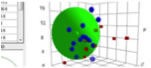
A simple example is the Sphere technique itself. On a SOM a good Sphere fit is equivalent to a (roughly) circular area of “good” molecules all separated from the rest of space which contains the “bad” molecules. In Hiroshi’s work on the new fitting regimes (Double-Sphere, Data…) he found that SOMs were very helpful in revealing problems with the datasets.

Here is an attempt to make the data fit a double sphere SOM. The lines are “guides for the eye” and not part of the SOM software output:

 

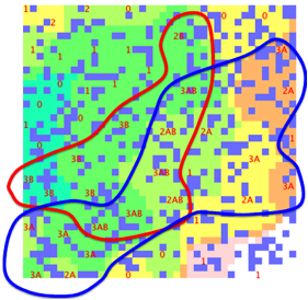
Figure 1‑3 A double-sphere SOM

Within this eBook we’ve already mentioned SOMs in terms of fragrance mapping. Such maps aren’t definitive about cause and effect, but they are suggestive of hypotheses which can be further explored.

Fitting

Another example from this eBook illustrates another way to explore. We were interested in the partition coefficient between soil and water, K_oc. It seemed reasonable to guess that the HSP distance between the chemical and some hypothetical soil would correlate with the partition coefficient. But what is the HSP of soil? The answer was to take a set of known K_oc values, make a guess at the HSP of soil, calculate the distances from each chemical and that soil and, by adding some further coefficients, predict K_oc from the distance. The square of the errors between predicted and actual values could then be summed – showing that the original guess, not surprisingly, was hopelessly wrong.

That’s when Excel comes in. Ask its Solver to minimise the error sum by varying the coefficients and the HSP of soil and see what happens. If the fit is still bad then the hypothesis is useless. If the fit is good then you have an effective working HSP for soil and can play around with some extra parameters (MVol or MWt usually have a part to play) to find the best fit with the least adjustable values.

If you have more sophisticated fitting algorithms then you can automatically find complex relationships which will give even better fits.

Once you’ve got some good fits it’s time to pause. Do the fits make sense in terms of basic chemistry and thermodynamics? Have you just found some meaningless relationship by providing too many fitting parameters, or does the relationship suggest some interesting science? Do the fits from the test data make good predictions for data not included in the fitting set?

The answers to those questions will vary. Sometimes the fits really are artificial and tell you nothing. Sometimes they fit so beautifully to standard HSP theory that you can be pretty sure that they are sound. But remember that the fits aren’t an end in themselves – they are a means to deeper understanding and, perhaps, useful predictions.

To boldly go

With the tools provided by HSPiP and with the extra tools in Excel (and other programs) it’s not hard to explore. Often, as with real explorers, the results are failures. But when the risks are small and the rewards are significant, maybe it’s worth having a go. We’ve used HSPiP’s tools for our own explorations and so made them as easy as possible to use. We hope you will want to use them for your own journeys into the unknown.

 

E-Book contents | HSP User's Forum