Chapter 30, DIY HSP (Methods to Calculate/Estimate Your Own HSP)

Life would be very easy if we had HSP of any chemical of interest to us. But as the number of published HSP is likely to be less than 10,000 and as there are literally millions of chemicals of interest the chances are small that you will find the numbers for your specific chemicals, though the 1,200+ chemicals we provide with HSPiP are a very good start.

So it would be very nice if there were a universally validated method for calculating HSP to a reasonable degree of accuracy. Unfortunately some of the methods require knowledge of other values such as enthalpy of vaporization or dipole moment and you may not know either or both of those.

The recent advances in statistical thermodynamics by Panayiotou and others offer some encouragement that HSP calculations will become more accurate and more routine in the years ahead. Similarly, work on molecular dynamics has proven fruitful in calculating δTot and recent work by, e.g. Goddard’s group in CalTech has shown tantalising evidence of being able to calculate δD, δP and δH. However, all these techniques are still only do-able in the hands of expert teams. So in the meantime we have to use a variety of approaches and, most importantly, our own judgement.

The most basic calculation is of δTot. This is simple:

δTot = (Energy of Vaporization/Molar Volume) ^½

But where do you find your energy (enthalpy – RT) and your molar volume? There are extensive tables of enthalpy values available at a price. Any modern molecular mechanics program can do a reasonable job of calculating molar volume and there are also free on-line tools.

So you might be lucky and be able to calculate δTot.

δP has been shown to be reasonably approximated by the simple Beerbower formula which requires just one unknown, the dipole moment:

δP=37.4 * Dipole Moment/MVol ^½

The more complex Böttcher equation (see equation 10.25 in the Handbook) requires you to know the dielectric constant and refractive index in addition to the dipole moment. It may arguably give better values if you have accurate values for all the inputs, but it is unlikely that you have those inputs so you are no better off.

The correlation has been re-done using the updated HSP list which, in turn was updated on the basis of the most recent databases of dipole moments. There is a necessary circularity to this process but the aim is self-consistency with all available experimental data so the process is highly constrained. The new fit, based on 633 values is shown in the graph:

 

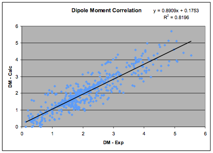
Figure 1‑1 The Dipole Moment correlation

and the revised formula, which is used in the HSPiP software is:

δP=36.1 * Dipole Moment/MVol ^½

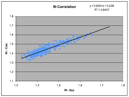
The paper by D.M. Koenhen and C. A. Smolders, The Determination of Solubility Parameters of Solvents and Polymers by Means of Correlations with Other Physical Quantities, Journal Of Applied Polymer Science 1975, 19, 1163-1179 does what the title suggests and finds not only an acceptable equivalent to Beerbower (they had an alternative power dependency for MVol but our revised data confirmed that 0.5 is optimal) but also a simple linear relationship between δD and refractive index. The coefficients shown here are our own fit to a more extensive and revised data set of 540 data points:

Figure 1‑2 The RI correlation

 

δD= (RI - 0.784) / 0.0395

Koenhen and Smolders also showed a strong correlation between δD²+δP², MVol^0.33 and surface tension. Using 498 data points with relevant surface tension data we found a correlation:

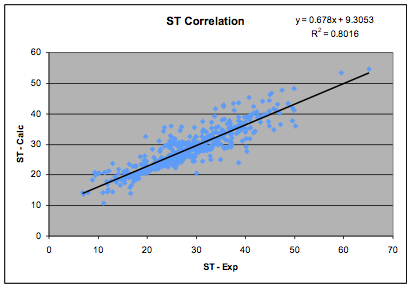
SurfTension=0.0146*(2.28*δD² + δP² + δH²)*MVol^0.2

 

Figure 1‑3 The Surface Tension correlation

 

When it comes to δH there is no obvious short-cut for calculating it from first principles using a few constants. We therefore have to rely on group contribution methods. And because we can use such methods for those, we might as well try to use them for δTot, δD and δP as well.

Group contributions

There is a long and distinguished history of breaking molecules down into a number of smaller sub-groups then calculating a property by adding together numbers for each group, weighted by the numbers of such groups in the molecule. There is an obvious trade-off in group contributions. It’s possible to define –CH2- as just one group or as 2 groups (-CH2- in acyclic and in cyclic molecules) or many groups (-CH2- in acyclic, in 3-member rings, in 4-member rings in 5-member rings etc. etc. etc.). The more subgroups used the more accurate, in principle, the group contribution but the less likely that there is sufficient statistical data to calculate the fits with any degree of reliability.

Over the years there has been a convergence on the so-called UNIFAC partition of groups – providing an adequate balance between over-simplification and over-complication.

So to calculate the group contributions for D, P and H one “simply” divides a set of molecules with known HSP into their individual groups then does a linear regression fit to the data at hand. In practice this is a lot of work and only a few such fits exist for HSP.

Because δD comes from Van der Waals forces it is intuitively obvious that group contribution methods should produce reasonable approximations. It doesn’t matter all that much where a C-Cl bond is as the more important fact is that there is both a C and a Cl.

δP is obviously problematic. A molecule with two polar groups near one end is likely to be more polar than one where those two groups are at opposite ends and tend to cancel out. It is hard for a group method to capture the geometrical issues.

Similarly, it is obvious that molecules with two –OH groups in them might differ strikingly in the amount of hydrogen bonding interactions between molecules depending on how much hydrogen bonding there is within each molecule. So δH can never be accurately determined from group methods.

So no matter how hard you try, you can’t realistically expect always to get accurate δH and δP values from group methods.

How does Hansen do it?

The overall goal is to divide the cohesion energy (Energy of Vaporization) into the three parameters discussed above. One finds or estimates the latent heat of vaporization at 25°C and subtracts RT (395 cal/mol or 1650 J/mol).

The preferred method to find δD is to use one of the figures in Chapter 1 of the Handbook. These give the dispersion energy of cohesion as a function of the molar volume. There are curves for different reduced temperatures. Use of reduced temperatures is characteristic of a corresponding states theory, which means that the HSP are based on corresponding states. The reduced temperature is 298.15/T_c. T_c is the critical temperature that can be found for many (smaller) molecules, but not for the larger ones. This then requires estimation. The T_c has been estimated by the Lydersen method as described in the Handbook using group contributions from the table for this purpose. T_c is found by dividing the temperature at the normal boiling point by the constant found from the Lydersen group contribution. One can then easily find δD with this energy and the molar volume. When this preferred procedure is not possible one can compare with similar compounds. Remember that δD increases with molecular size, especially for aliphatic molecules. This combined with the probable incompatibility of group contributions with a corresponding states theory makes the accurate estimation of δD especially difficult, especially for polymers.

δP is usually found with the Beerbower equation given in the above, or else by group contributions as reported in the Handbook. If a dipole moment can be found for a closely related compound, its δP can be found with its molar volume, and this can then be used to find a new group contribution value for use with the table in the Handbook. This procedure is best when the whole procedure of finding HSP values is possible for the related compound. The ultimate result is two new sets of HSP.

δH in the earliest work was found exclusively by difference. The polar and dispersion cohesion energies were subtracted from the total cohesion energy to find that left over. This was then used to find δH. When things did not add up properly comprises were made based on the multitude of experimental data that were generated in the process of establishing the first values. Up to the point where the Panayiotou procedure came forth, the usual method of estimating δH was with group contributions as given in the Handbook.

For the sake of historical record, note that the original values reported by Hansen in 1967 were expanded to a total of about 240 by Beerbower using the Böttcher equation, his own equation, and the group contributions in the tables in the Handbook. This set was then extended over the years by one method or another by Hansen to arrive at the values found in the Handbook. The revision process will presumably continue, but the original values from 1967 seem to be holding up well. The Hoy parameters are not compatible with the Hansen parameters, particularly with respect to finding a dispersion parameter that is too low. The Van Kevelen procedure also gave somewhat inconsistent values and did not have a wide selection of groups to use. Experimental data were found where possible and practical, and adjustments made accordingly, but one must do this with care, since what looks good in one correlation may totally ruin another.

Much better than nothing

So now you know the bad news about DIY HSP. There is currently no good way to be sure you have calculated accurate values, for reasons which are fundamental. So, do we abandon hope?

Happily the answer is that by using all the available methods and combining them with your own scientific understanding, it’s possible to get HSP that are fit for purpose. If the molecule is well outside the sphere it doesn’t really matter how far outside it is. So it often doesn’t matter if δH is 12 or 14. It suffices for you to know that it’s not 2 or 4.

And if you find that it’s critical to know if δH is 12 or 14 so that you can really refine the radius of the Sphere, you can resort to good old-fashioned experiment to get the HSP for the one molecule that happens to be of critical importance.

The 6 ways

In the program we offer you 6 ways to calculate HSP.

1 This lets you input enthalpy, molar volume, refractive index and dipole moment. You therefore get δTot and δP. If you also enter an estimate for δD the program calculates δH. You can also correct for temperature of calculation of enthalpy and see an estimation of the surface tension from your calculated parameters.

2 The most extensive and accurate published group-contribution method for all 4 values (δTot, δD, δP and δH) comes from Panayiotou’s group in Aristotle University in Thessaloniki. The Stefanis-Panayiotou method (E. Stefanis, C.Panayiotou, Prediction of Hansen Solubility Parameters with a New Group-Contribution Method, International Journal of Thermophysics, 2008, 29 (2), 568-585) has established itself as an important method. The extra feature of S-P is that it attempts to distinguish different forms of similar groups by identifying 2^nd-order groups which have their own parameters. If you want a rough estimate, then keep things simple and ignore the 2^nd-order groups. For more accuracy you must include the 2^nd-order groups. It can be difficult to know how to partition your molecules into these UNIFAC groups. Helpfully, S-P provided an example of each type of 1^st- and 2^nd-order group to help you break down your molecule in the correct manner.

A typical example is 1-Butanol which has 1 CH3- group, 3 –CH2- groups and one –OH group. If you enter these (1^st-order) values and press calculate you get values for δTot and then δD, δP, δH of 21.9 and [15.9, 5.9, 13.2] (c.f. [16, 5.7, 15.8]) respectively.

There is a further refinement. If you are confident that the molecule (for whatever reason) will tend to be of low δP and/or δH, you can click the “Low” option and use group parameters tuned for these respective properties. To help you with your intuition, if you attempt, for example, to use the Low H option for 1-Butanol you get a warning because there is not (should not be!) a Low H fitting parameter for this molecule.

For users who aren’t too comfortable in creating the UNIFAC groups, the Y-MB method below provides an automatic way of creating these groups (first-order only) from Smiles or 3D molecule input. No automatic group method can be 100% accurate so you need to do your own sanity check, but in our tests it has proven to be most helpful. It’s also insightful to compare the HSP predictions of the two methods – they both have their strengths and limitations.

3 Van Krevelen is the first to admit that his group method cannot give accurate results, for the reasons discussed above. His particular contribution to the problem is to introduce a “symmetry” option. If there is one plane of symmetry then the polar value is halved, with two planes it is quartered and with 3 planes both the polar and hydrogen bonding values are set to zero. The one-plane choice, for example, would help distinguish our two cases of C-Cl bonds discussed above.

4 Hoy uses a more subtle form of calculation from his chosen groups and includes options similar to Panayiotou’s secondary groups by taking into account various x-membered rings and some forms of isomerism. Importantly, Hoy also attempts to make corrections for polymers. It’s intuitively obvious that, for example, the polar effect of an isolated sub-unit would be rather different from the overall polar effect from the polymer chain made up from those sub-units.

Hoy also helps with input to the numerical and Van Krevelen calculations by producing an approximate value for the molar volume. This can’t be as accurate as a proper measurement from density and molecular weight or from a molecular mechanics program, but it’s a useful aid if you can’t derive it from those sources.

5 One of the issues with group methods is that they often can’t satisfactorily predict complex inter-group interactions. Hiroshi Yamamoto therefore adapted his Neural Network (NN) methodology for fitting the full HSP data set  in such a way that inter-group interactions automatically get fitted by the relative strengths of the neural interconnections. But of course this needed him to have a set of groups. He therefore devised an automatic Molecule Breaking (MB) program that created sub-groups from any molecules. He used a general MB technique that allowed him to experiment with which combination of MB and NN gave the best predictive power for HSP. That’s what you get with HSPiP. And because the MB technique was general, he was able to take standard molecular inputs (such as Smiles, MolFile (.mol and .mol2), PDB and XYZ) and "break" them so the user can get completely automatic calculation of individual molecules (plus their formula and MWt) or, given a table of Smiles chemicals, bulk conversion to a standard .ssd file with a large set of chemicals. [If you happen to have a set of chemicals in another format, such as Z-matrix, which HSPiP cannot handle, then we recommend OpenBabel, the Open Source program that provides file format interconversion for just about anything that’s out there. We used OpenBabel a lot when we were developing the implementation of Hiroshi’s technology]. Charles and Steve have called the method Y-MB for Yamamoto Molecular Breaking [Hiroshi was too modest to want such a name] and we believe that Y-MB represents a fundamental change in the way HSP can be used in the future. Hiroshi’s extensive knowledge of Molecular Orbital (MO) calculations and their interpretation means that in the future Y-MB might be augmented via MO.

In addition to the HSP values, Y-MB provides estimates of many other important parameters such as MPt, BPt, vapour pressures, critical constants and Environmental values.

Like all group contribution methods, Y-MB isn’t magic. It can’t accurately predict values for groups or arrangements of groups that are not in its original database. The more HSP that can be measured independently, the more Hiroshi can refine the Y-MB technique to give better predictions. As mentioned above, the Y-MB breaking routine can optionally find the Stefanis-Panayiotou UNIFAC groups.

For the 3^rd Edition, Hiroshi carried out a huge analysis of results on a database of many thousands of molecules including many pharma, cosmetic and fragrance chemicals. From this he was able to refine his list of group fragments and also test novel NN and Multiple Regression (MR) fits. As a result we now have internal NN and MR variants for calculating the different parameters of Y-MB. Each has its own strengths for different properties. For the user the only difference from previous editions is that the estimates are often improved – particularly for very large molecules where we acknowledged that the original Y-MB had problems.

Because we believe that the relatively new InChI (International Chemical Identifier) standard for describing molecules is going to be of great future importance, we output the “standard” InChI and InChIKey. These are created with the “No Stereochemistry” option so they are the simplest possible outputs. Importantly, if you use the first 14 digits of the InChIKey as the search string on places such as ChemSpider (probably the best one-stop-shop for information on a chemical) then you are guaranteed to get the correct matches. InChIKeys are unique identifiers created from the InChI so unlike CAS# they are directly traceable to specific molecules and there is only one InChIKey (well, the first 14 digits) to a molecule. The reason we emphasise the first 14 digits is that they will find all variants of a given molecule, independent of stereochemistry, isotope substitution etc. Once you start using InChIKeys for searches you’ll wonder how you ever survived without them.

For a useful quick guide to InChI, visit http://en.wikipedia.org/wiki/International_Chemical_Identifier

6 Polymers are a problem. We have no reliable general method for predicting polymer HSP. This is not surprising. For example, there is no such thing as “polyethylene”; instead there are many different “polyethylenes” and it would be surprising if their HSP were all identical. But that doesn’t mean that we should give up. An intelligent estimate can often provide a lot of insight. Hiroshi had proposed an extension of his Y-MB technique to include polymers. And by good fortune we found Dr W. Michael Brown’s website at Sandia National Laboratories:

http://www.cs.sandia.gov/~wmbrown/datasets/poly.htm

With great generosity, Dr Brown gave us permission to use his dataset. Hiroshi then implemented a revised version increasing the number of polymers from <300 to >600. To make it more consistent with the rest of the program we’ve used –X bonds as symbols of the polymer chain rather than the pseudo-cyclic “0” used by Dr Brown.

To calculate the polymer HSP, simply double click (or Alt-Click) on one of the polymers. This puts the Smiles up into the top box. Then click the Calculate button as normal. You can, of course, enter your own polymer Smiles manually if you wish.

As the whole area of polymer HSP prediction is so new, the Y-MB values for a single monomer repeat can often be somewhat unreliable. You can, therefore, set a number of repeating units, say, 4, and the full polymer Smiles for this 4-mer is created and the Y-MB values calculated. You can use your own judgement as to which value to use – the 1-mer, 2-mer, 3-mer … There are some complications to this automated process. If, for example, you had a 2-ring monomer and asked for a 5-mer, you will get a message to say that this is impossible – the problem is that the first rings would be labelled 1,2, the second 3,4 and the 5^th repeat unit would be 9,10 – and polymer Smiles can only use rings from 1-9.

Although this is hugely helpful, we think there’s even more that can be done with this. With a bit of intelligent copy/paste you can construct polymer blends. For example, if you take polyethylene, C0C0, and polycyclohexylethylene, C0C0C2CCCCC2, you can combine them to create the ABAB copolymer C0CCC0C2CCCCC2, or the AABBAABB copolymer C0CCC CC(C2CCCCC2)CC0C2CCCCC2 etc. It’s a bit tricky (note the extra parentheses around the middle cyclohexyl group) but it’s pretty powerful. To help you we’ve added a CP (Co-Polymer) button that you can click when you’ve selected two polymers from the database. The program automatically creates an AB, AABB or AAABBB polymer according to your choice. Note that it is possible to make “impossible” polymers this way – the program makes no effort to see if two monomers could actually be made into a co-polymer.

Again we need to stress that this is all so new that the predicted values should be treated with caution. Above all we need many more experimental data points for polymers and it seems that IGC offers a lot of hope for the routine gathering of a lot of relevant data. Armed with more data, the polymer Smiles predictions can be refined.

We had pointed out to users of the Polymer Smiles method in earlier editions that the limitations were significant. With the improved Y-MB version we are much happier that Polymer Smiles are more stable and insightful. They should still be used with caution, but their capabilities are clearly much improved for the 3^rd Edition.

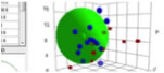
If you want to see the structure of any of the polymers, Ctrl-Shift-click on the polymer in the database and a 3D representation appears in the Y-MB tab. We created the 3D structures automatically from the polymer Smiles using the public domain OpenBabel utility.

Revisions to the HSP table

We’ve used all the above considerations to update the HSP data used in HSPiP. Many of the changes have been minor, some will be more significant. Any changes will be unwelcome to those who have been using the Hansen table for years. So it’s worth explaining why we made the changes.

There is a fundamental principle that all worthwhile databases contain errors. The published Hansen table contained a few typos, and a few errors. But many of the changes have come about because the basic data in other databases such as DIPPR 801 and Yaws' Handbook of Thermodynamic and Physical Properties of Chemical Compounds have changed. Thanks to Hiroshi Yamamoto we were able to carry out a systematic comparison of the δTot with the published total solubility (Hildebrand) parameters. We could then see if it was reasonable to change any values using dipole moment and refractive index data contained in those databases. The fundamental principle of databases means that those databases also contain errors and conflicts. Wherever possible we corrected those molecules where there was a large (>1) difference in δTot, but used the principle of least change if DIPPR and Yaws disagreed, and used the principle of common sense when a value in those databases simply made no sense.

We have continued to work with Hiroshi to challenge and revise the HSP database, especially when any fresh data appeared. We continue to be hopeful that  new measurements of HSP (e.g. via IGC) will start to accumulate. See the next paragraph for how you can help!

DIWF

The alternative to DIY is Do It With Friends. The .hsd format is a simple text format that makes it very easy to exchange HSP values. If members of the HSPiP user community email to Steve their HSP values for chemicals not included in the official Hansen list then we can start to share them amongst the community. Although each individual user might be losing out by giving away some hard-won data, the community as a whole will benefit. When different users come up with different values, we can choose to quote both or launch a discussion to decide which is right.

Indeed, it might be time for those with their private collections of HSP to open them up to the world-wide HSP community. Of course they would lose some commercial/academic advantage by revealing their values. But they would also gain by having those values corroborated and/or refuted by values from other collections. By assembling one large “official” HSP table, with differences resolved by expert assessment, many of the glitches and problems in the literature and in our own practical research enterprises would disappear. Will readers of this book take up the challenge? We hope so!

 

E-Book contents | HSP User's Forum