Chapter 33, Into the 4th Dimension. Donor/Acceptor

We would like to warmly thank Professor Michael Abraham, University College London, for his generous assistance with respect to his Abraham parameters.

As we’ve noted in other chapters, there are other approaches to determining solubility. Each has its strengths and limitations. Here is our view, in alphabetical order, of some of the main approaches.

Abraham parameters. For more than 20 years, Professor Abraham and his team have methodically worked out a set of 5 parameters that allow users to calculate solubilities and partition coefficients based on linear free energy relationships. The parameters have been worked out through careful, complementary experimental processes using solvatochromic shifts, NMR shifts, GC and HPLC retention times. The approach has been adopted in a number of areas and the large experimental database of parameters is a key aspect of the approach. We will discuss the parameters later in this chapter.

COSMO-RS. Dr Andreas Klamt has developed an entirely new way of working with solubility and partition issues. At the heart of the technique is quantum mechanical calculations of each molecule (and, sometimes, each major conformer of the molecule). Once the calculated data for the molecule is known, subsequent calculations of interactions with other molecules are rapid. In principle, therefore, COSMO-RS can do everything that all methods try to do, but can do it from first principles. There is no doubt that this approach is very powerful. As the base of validated quantum calculations increases the usability for everyday problems will increase. For the purposes of this chapter we note that COSMO-RS is able to generate “COSMOments” and a 5-parameter set which we will discuss below.

MOSCED. MOSCED’s roots are not too distant from HSP. At an early stage it was recognised that increasing the number and complexity of parameters would provide better fits to the data. In particular, MOSCED introduced an acid/base split of parameters to recognise specific interactions such as acetone/chloroform. MOSCED becomes, therefore, a 5-parameter set. Recent MOSCED papers have shown excellent agreement with activity coefficient data. However there does not seem to be a robust set of MOSCED parameters for general use and it is unclear to us how the current MOSCED parameters relate to the cohesive energy density that is at the root of the concept.

UNIFAC and its variants. If you are a UNIFAC user then you probably aren’t reading this eBook. UNIFAC’s strengths are unparalleled in its main domain of use for vapour liquid equilibria in the chemical industry. However it doesn’t seem to have caught on as a tool for the broad range of applications for which HSP are so suitable. There is now a huge database of UNIFAC group coefficients and if you have access to the database you can do many things better than you can with HSP.

If we leave out UNIFAC as a special case, it’s clear that other methods have 5 parameters whilst HSP has only 4. Why 4 – surely HSP has only 3 parameters? In this chapter we’ll emphasise the fact that HSP calculations regularly use the MVol. MVol has appeared in all HSP data tables and has been quietly working away in the background. The other 5 parameter sets also include a term that is equivalent to MVol.

An important paper, Andreas M. Zissimos, Michael H. Abraham, Andreas Klamt, Frank Eckert, and John Wood, A Comparison between the Two General Sets of Linear Free Energy Descriptors of Abraham and Klamt, J. Chem. Inf. Comput. Sci. 2002, 42, 1320-1331, shows that the Abraham approach and a simplified version of COSMO-RS (COSMOments) can both be described by a 5-parameter set which can be adequately mapped between the two techniques. This paper, incidentally, is an excellent introduction to both approaches and is recommended for those who want to understand more about them.

For the purposes of this chapter, the paper can be summarized by saying that the HSP terms of δD, δP and MVol map onto corresponding terms in both Abraham and COSMOments. But δH is a single term whilst Abraham has Acid/Base and COSMOments has H_donor and H_acceptor. The mapping of Abraham Acid/Base onto COSMOments H_donor/H_acceptor isn’t perfect – after all the other parameters aren’t perfect maps – but the paper makes the point that the general idea of a 5-parameter linear free energy space is a core thermodynamic concept.

Because it is clear that both Abraham and COSMOments work well with extensive experimental databases it means that HSP has to defend its use of a single δH parameter.

There has been no shortage of suggestions that HSP should divide the δH parameter and there have been a few attempts to make it happen. But there have been three practical objections. The first is that the 4-parameter HSP (remember, we are including MVol as a parameter in this chapter) works remarkably well. The second is that plotting in 4D space (δD, δP, δHD, δHA) isn’t possible in this 3D world. The third is that there’s been no obvious way to partion δH into the two terms.

But the classic acetone/chloroform case where there is unambiguous evidence of donor/acceptor interactions between the solvents shows that 4-parameter HSP cannot describe everything. However, as noted in Charles’ history in the next chapter, even this case doesn’t show up as special in general HSP use.

Acid/Base or Donor/Acceptor

Sooner or later we have to decide on terminology. The world is split into those who think that the best term to describe the two terms is Acid/Base and those who think it should be Donor/Acceptor. As you can see above, Abraham and Klamt use respectively Acid/Base and Donor/Acceptor.

We decided that Acid/Base is rather too literal so have chosen Donor/Acceptor. Hence we will talk of δHD and δHA rather than δHA and δHB. The fact that the A of Acceptor is the opposite meaning to the A of Acid is unfortunate, but there’s nothing we can do about it.

While we are clarifying terminology, let’s restate that we talk about a 4-parameter or 5-parameter set but a 3D or 4D viewing space. This is because the (scalar) MVol is not shown in the (vector) plots of 3D or 4D space.

Inspired by Abraham

Reading the extensive publications of the Abraham team and examining their large public database of parameters it is clear that their thoughtful approach to working out the Acid/Base parameters is much to be admired. The IGC and HPLC techniques for HSP were developed independently of the equivalent Abraham GC and HPLC work and show that in principle the Abraham parameters could map onto an HSP 5-parameter set or, to put it another way, HSP could in principle (though this won’t happen in practice) gather Donor/Acceptor values in a similar fashion.

We therefore decided to create a 5-parameter HSP set using Abraham parameters to help us in one important step. We decided to split δH using two rules.

Rule 1:     δH² = δHD² + δHA²

This rule ensures that everything about HSP stays constant and we can always bring Donor/Acceptor back into 4-parameter space without upsetting 40+ years of work.

Rule 2: For compounds with known Abraham Parameters, δHD:δHA = Abraham Acid:Base

This rule allows us to get started on the whole process of rationally splitting δH. We have no pure scientific justification for this mapping other than our feeling that the Abraham approach to Acid/Base determination (e.g. GC/HPLC) fits very well with HSP.

Once we were up and running with a basic set of Donor/Acceptor splits, it was then possible to create Y-MB methods for splitting molecules for which we had no Abraham parameters.

After that it requires a lot of checking and invoking chemists’ common sense. If the automated process produced an amine with a large δHD then clearly there was a problem with the process.

Out of this work came an important third rule:

Rule 3: If you have no other way to decide, make δHD=0 and δHA=δH.

This surprising rule is less surprising if you glance at any Abraham table. For example, in a table of 500 compounds there are 466 with Base values and 249 with a Acid values. And of those 249, only 96 have a value bigger than the Base value. So most molecules are Acceptors rather than Donors. Of course Rule 3 should be used with care but note that it says “if you have no other way to decide”. If a molecule has a carboxylic acid group then you already know something so Rule 3 doesn’t apply.

Calculating the distance

The previous section describes in a few words a very large amount of work. This section describes some hard thinking.

 

When 5-parameter HSP seemed only an impossible dream we assumed that if we had them it would be easy to calculate the HSP distance. MOSCED, for example, uses (in our nomenclature) a term (δHD₁-δHD₂)(δHA₁-δHA₂) instead of (δH₁-δH₂)². This term captures the possibility of a “negative distance” which is what Donor/Acceptor is supposed to accomplish.

However, we quickly found that we cannot use such a term. If the two donor terms are equal then the first term is zero so the distance is zero. But this cannot be the case for HSP. For example if δHD₁ and δHD₂ are both zero then the second term should be equal to the classic δH distance because each δHA term equals the classic δH.

We eventually found a distance formula that works well. It gives the sorts of values we intuitively expect in all the test cases we can find. We would love to be able to tell you that we understand the reason for the formula, but we admit that we use it because (a) it seems intuitively right and (b) it is the only formula out of many variants that gave us only values that made intuitive sense. If someone from the HSPiP user community can prove it or provide a better alternative we would be happy to acknowledge their work in a future edition.

So if we have (δHD₁ , δHA₁) and (δHD₂ , δHA₂) then using the nomenclature Min(X,Y) to mean the minimum of X or Y, we define:

Equ. 1‑1 MinX1 = Min(δHD1 , δHA2)

Equ. 1‑2 MinX2 = Min(δHD2 , δHA1)

Equ. 1‑3 X1 = δHD1 - δHA2

Equ. 1‑4 X2 = δHD2 – δHA1

Equ. 1‑5 S1 = δHD1 - δHD2

Equ. 1‑6 S2 = δHA1 - δHA2

Equ. 1‑7 DA1 = Min(δHD1, δHA1)

Equ. 1‑8 DA2 = Min(δHD2 - δHA2)

Then

Equ. 1‑9 Distance = -Sqrt(MinX1²+MinX2²) + Min(Sqrt(X1²+X2²), Sqrt(S1²+S2²))+Sqrt(DA1²+DA2²)

If both δHD values =0 or both δHA values=0 then this term becomes the classic (δH₁-δH₂)²

If δHD₁ is large and δHA₂ is large while δHD₂ is small and δHA₁ is large then we have a classic donor/acceptor (chlororform/acetone) pair and the distance is negative, which is precisely what we require. Mathematicians will note that when we calculate the Distance²  (in the general distance formula) Distance² =Sign(Distance)* Distance².

Most other cases show some reduction in distance from the classic δH distance because of some favourable donor/acceptor interaction.

It’s worth noting that although there are a large number of molecules with a high δHA and a low (or zero) δHD there are very few molecules (<5%) with a δHD more than twice δHA, and only 2% with more than 3* δHA. So the likelihood of strong pure Donor:Acceptor effects is very low.

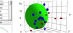
Our first 4D Spheres

We were very nervous when we created our first Spheres using standard .hsd files (and therefore known classic Spheres). What would happen if the results were very different. Would this mean that 40 years of HSP have been wrong?

We needn’t have worried. It quickly became clear that for most systems the results were not very different. There are three very important reasons for this. The first is obvious: because δD and δP have not changed, it’s not possible for the Sphere to move too far. The second reason follows from the facts behind Rule 3 above. Because a large majority of molecules have a very low fraction of Donor, the majority of interactions are Acceptor:Acceptor, in other words they are simply classic δH. The third is simple statistics: the number of systems with large δH values isn’t large and the effects of a Donor/Acceptor split from a small δH value is not highly significant.

But the fact that they are not very different doesn’t mean that the whole 5-parameter approach is a waste of time. In some cases the fits improve because there really are specific Donor/Acceptor interactions for a few solvents and a few polymers, particles etc.

For us, and we think for you, the move into 5-parameter space is a useful option. For most work, the proven 4-parameter methodology works very well and there is no need to add the complexity of the 5-parameter space. But given that we can create the Donor/Acceptor split automatically and that the Sphere fitting isn’t too much slower, it’s easy to explore the option if there are reasons to expect that Donor/Acceptor effects will be large. And remember that “more” isn’t always “better”. The split adds extra uncertainties to parameters which themselves have errors. It is possible to make things worse by trying to be too clever. So we recommend that for routine use, the 4-parameter classic method should be your default. But feel free to enter the 4^th dimension at any time.

Reporting the results

Because we cannot plot a 4D Sphere and because of Rule 3 above, we will continue to plot the classic Sphere. So δH will always be calculated for you from δHD and δHA via Rule 1 and plotted as normal. But of course we show you the δHD and δHA values in a table so you can understand what is going on with each of the solvents.

We cannot save 4D data in the old .ssd file format. The new, standard, more versatile .hsd format is equally happy with 3D and 4D data.

The problem of mixtures

One of the great strengths of HSP is the ability to create arbitrary mixtures and calculate the HSP by the standard mixing rule. Things get more complicated when solvents are blended with Donor/Acceptor.

As an extreme example (which, see the comments above, is highly unlikely to exist), suppose we have a 50:50 blend of [10,0] and [0,10] – the mixture of an equally strong pure donor and pure acceptor. In δH terms the classic answer is 5+5=10. One possible intuition is that the donor/acceptor cancel out giving [0,0]. But it seems unlikely that the resulting blend would have no δH. It also seems unlikely that it would be [10,10] with a resulting δH of Sqrt(10²+10²)=14.14. After much experimentation we found that the simplest possible mixing rule, the weighted average of δHD and δHA terms, gave sensible and intuitive results. In this example the answer is [5,5] with a total δH of 7.07. Most other cases aren’t so extreme and the resulting δH is not much reduced from the simple weighted average of δH terms.

An alternative possible rule is that δH of the mix remains the same as the classic mixing rule, but the ratio of δHD and δHA is changed depending on the relative values of the components. This is a slightly more complex rule to implement and in most cases makes little difference, so for the moment we have chosen the simple rule.

Because so much of this is provisional, we’ve decided not to include donor/acceptor into the Solvent Optimizer.

Activity coefficients

In other chapters we have pointed out that activity coefficients should be directly calculable from HSP distance. But there is lots of experimental evidence to show that this is not a reliable method for prediction. Clearly the impossibility of a negative distance, indicating a Donor/Acceptor interaction, has been a limitation of the 4-parameter HSP.

For this release of HSPiP we simply haven’t had the time to do the vast amount of work to see if a 5-parameter model gives more reliable predictions. That is something for the next release.

Use with care

We believe that this shift to a 5-parameter HSP is a necessary step in the evolution of HSP. But our evidence is that the step is in most cases not of great importance. So classic HSP has not suddenly been invalidated. Therefore we are not shifting everything at once. On the surface, much remains 4-parameter, though behind the scenes we use 5-parameter when it seems sensible. Unless you select the D/A option you won’t even see the 5-parameter data.

We have some internal cases where the Donor:Acceptor correction is so large, and the δD and δP parameters are so close that the distance is negative, though without an especially high solubility. In other words our formula seems to over-correct in some cases. We will carry on our internal arguments on the issue while this current edition is out in the open. We very much look forward to your input to the debate.

But the key take-home message here is to “use with care”. It’s possible that we will change the Distance algorithm and the Mixing algorithm. Our splitting ratios may change with time as we gather more experimental data. So enjoy exploring the 4^th dimension, take what value you can from it, but, at this stage, don’t rely too heavily on its predictions.

 

E-Book contents | HSP User's Forum