How to use Solvent Optimizer

You may have found a great solvent for your system but it is too toxic or expensive to be used in your application. No other single solvent is good enough. Or you may have a polymer for which you want to find a good solvent mixture. In both cases you click the O Optimizer button and the Solvent Optimizer form appears with the HSPs of your great solvent or your polymer automatically set as the Target for your optimization.

 

 

You can, of course, enter values manually into the target and add a Radius value for use in various calculations.

 

The aim is to find a mix of solvents that closely match your target. Note that the mix within Solvent Optimizer is expressed in terms of Volume %.

 

The Distance from your solvent to your target is automatically calculated and, of course, you can sort the solvents by this distance by clicking on the column header. This is a very easy way to identify the closer solvents.

 

The default solvents that appear in the Optimizer are “friendly” solvents – ones that are well-known to be cost effective, much used, less harmful, requested by HSPiP users, etc. (though not necessarily all three). You can edit this list from within the program (recommended) or by directly editing the file OptimizerSolvents.sof (but make sure you keep a backup!). You can also Load/Save any number of .sof files to suit your own purposes.

 

 

Shipped with the program is a file called NoAlcohols.sof which is simply the standard list with the weighting (see below) of those solvents containing alcohol functionality set to 0%. Similarly there are files related to cosmetic/pharma needs such as PermeationEnhancers.sof. If you select the P. Load/Save option then your parameter sets are loaded/saved. This is an option because sometimes you don’t want to override your current settings when you load a different .sof file, though it’s probable that you will want this option set to its default “on” setting most of the time.

 

If the XC option is selected then eXtra Columns of data appear – for BPt, FlashPt (in °C), VP@25°C, MPt and MWt. These values are supplied in the DefaultSolventOptimizer dataset and are also copied over from the Master Dataset if the Right-Click trick (next paragraph) is used. These values are provided for convenience only – the SO does not use them in any way. It is the user’s responsibility to check that the data are accurate – especially for FlashPt which has legal ramifications for safety.

 

You can also transfer solvents from the main tables to the Solvent Optimizer. Select one or more solvents by clicking (or Shift-clicking or Ctrl-clicking, as per any Microsoft-style table) on the “selection” box on the left-hand edge of each solvent in whichever main table you want to get them from, then Right-Click on the text of one of the selected lines and, after a message appears for you to confirm that this is what you want to do, the solvents will be added to the Optimizer.

 

Some users like the option of loading an .hsd file into the Optimizer or to save an Optimizer file as a .hsd for importing into the main Sphere program. To do this, click the Convert button before clicking the Load/Save buttons.

 

Data specific to each format is lost during conversion – you only preserve the names, HSP and MVol parameters, though during Load an automatic lookup checks if the name matches the name in the master database and imports the RER and Antoine data. Clearly this feature won’t work if you call your solvent Dimethyl Ketone instead of the name Acetone which is used in the database. The Convert option automatically unchecks itself so that you don’t accidentally lose data if you subsequently save a .sof file.

 

The fastest way to getting some good ideas is to press the 2 button which finds the Best Pair of solvents. The program examines all possible combinations of two solvents and finds the mix with the closest match to your Target (i.e. the smallest HSP distance defined in the usual manner using the factor of 4 weighting for D values). You get a list of the Calculated values, the Deltas between the Target and the best pair, plus the Distance which is the optimized HSP distance from the calculation.

 

This pair of solvents may be OK. But it may not be quite what you want. You can then start to “play”. For example, select a third solvent by clicking the relevant checkbox. Then press the O Optimize button. This now finds the optimum proportions for the three solvents.

You can do this for a maximum of 10 solvents. Up to 5 solvents calculations are quite fast. For 6 solvents things slow down a lot. For 7 or more solvents the accuracy is reduced to bring the speed close to that of 6 solvents.

 

To help you find solvents we’ve implemented a clever idea suggested by one of the HSPiP community. If you select Show Hi-Lo then each entry in the table is coloured red if it is higher than the Target value and blue if it is lower.

This makes it much easier to spot pairs of solvents which must have complementary hi/lo values in order to result in a match to the target. Hi-Lo is not shown for Donor/Acceptor as it would require multi-coloured options.

 

The Best 1 or 2+ option allows you to specify an extra distance (e.g. +0.5) so that when you click the 2 button (this also applies to the 1 button described below) not only do you get the best blend but you get a list of blends which are within your chosen extra distance from the best blend. This list is placed on the Clipboard ready to paste into, e.g. Excel.

 

This capability is very useful. When you get an automatic optimum blend you don’t know if this is much better than alternatives or is within a few decimal points of many others. By looking at the Best+ list you can quickly identify blends that are good enough but, perhaps, with solvents that you prefer.

 

Alternatively, you can simply select any solvents you like and enter their % manually. At any time you can click the Calculate button. If the % don’t add up to (close to) 100% then the calculated values are shown as “err” to warn you that there’s an error. You see the calculated total % shown in red. You can then easily fix the problem. As the last few % may not be too critical, the program calculates an answer if the total % adds up to between 95 and 105%. Obviously you should look at the % Check value to make sure you get to 100%.

 

 

There are two further options. The 3 button automatically finds the three best solvents. This can take some time if you have a lot of solvents, so be patient. The 1 button has two uses. Suppose you absolutely must use a specific solvent and you simply want to find which one other solvent in the list, at what ratio, gives the best match to the target. In this mode you simply make sure that the check-box is ticked for your solvent, with no % value. Clicking the 1 button finds the best other solvent.

 

The other use for the 1 button is when you know that you must use X% of some solvent and, perhaps, Y% of another solvent and want to find one other solvent (at 100-X-Y%) that gives a good match. In this case, select the solvent(s) you want and enter its/their % values. Clicking 1 finds the best solvent to make up your blend.

 

As described above, the Best 1 or 2+ option allows you to find other single solvents within your specified extra distance, in case the best one happens to be only marginally better than an alternative with a solvent you happen to prefer.

 

The Pw (PairWise) button is for those who need an exhaustive search for the best ratio of each of the possible pairs of solvents from the list. Why would you want this? One example is to make sure that you know not only which individual solvents are within a chosen distance (you find that from the Distance column) but which pairs of solvents (at their optimum blend) are within a chosen distance. This would tell you, for example, all possible solvent pairs that could dissolve a given polymer. Clicking the Pw button does an exhaustive search of all such pairs then sorts the output before placing it on the Clipboard. The output (which is often too large to be of much use within HSPiP) can then be pasted into something like Excel for further processing. Note that redundant pairs are removed. So if your list contains Acetone and Xylene, the Acetone:Xylene pair will be shown but not the (identical) Xylene:Acetone pair.

If you first select 4 or more solvents then click Pw, you get the pairwise combinations of just those selected solvents.

 

Tw is the Triplet-wise equivalent. Because this would give vast numbers of combinations, this works only if you have selected 4 or more solvents.

 

Each time you do a calculation, the results are automatically sorted in descending order of % solvent. This conveniently groups solvents together for you, otherwise it can be difficult to see what is going on.

 

For those who like to explore the world of split δH, the D/A option shows the δHdonor and δHacceptor values and optimisations use these values instead of δH alone. The formula used for blends and for distances is via simple summation. This is certainly not the scientific ideal, but until that ideal is properly understood, the simple summations are at least indicative of Donor/Acceptor trends.

 

For a permanent record, click Capture Screen to Clipboard camera. You can then paste the image into Word etc.

 

When you press the Copy to Table button, your target, the deltas and the solvents are all placed onto the Clipboard for convenient pasting into Word/Excel. There are two of these buttons. The S version copies only the Selected solvents. The A version copies All the solvents – use whichever is more useful to you. In both cases, your current parameter settings are included in the copy.

 

If you just want a simple printout of your table then click the Print Table button. If you want fancier printing then use Capture to Table to place the data in Excel and use the many options there for fancy print formatting.

 

Polymers that match the Calculated values

Clicking the P button opens the Polymers form, with the polymers sorted according to their closeness to the Calculated values.

 

If these aren’t valid (e.g. because % values are wrong) then the Target values are used instead.

 

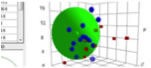
Viewing the Solvents and Target

By clicking the Sphere icon you get a 3D plot on the main form of your optimizer solvents and the Target.

 

The radius of the Target is set by the Double-Click R on the main form. What you see depends on your choice of view on the Sphere form. To see just your chosen solvents, select “In only”, to see them with their names, select “In + Name” and so forth. If you select “In + No.” the number is simply the row number of the solvent. You can change the view till it shows you what you want to see. The colour codings/shadings are as in Sphere: a solid blue sphere means your chosen solvent is inside the sphere, an open blue sphere means your chosen solvent is outside the sphere and so forth. The “Min” options don’t apply to this view. No calculations are done – this is simply an option to view the solvents in this context.

 

Weighting

If you want to discourage (but not totally exclude) the use of one or more solvents, then you can lower their Weight value from 100%. A value of 50% will be reasonably discouraging, a value of 0% will be strongly discouraging.

 

This can help you include other considerations (such as solvent cost) in your optimization.

 

The weighting function simply adds an extra “distance” to the calculations, depending on the % of the weighted solvent and its weighted value. You can see the value of this extra distance in the Weight error box. A large value means that the optimization is fighting hard to avoid using your weighted solvent(s) but doesn’t have a good alternative.

 

Temperature Effects

There is a little-known phenomenon of polymers having reduced solubility at higher temperatures. This can come about because a well-matched solvent can change its HSP with temperature and become mismatched to the polymer. This in turn happens because the thermal expansion coefficient of the polymer is much less than that of the solvents. By clicking the ºC button the temperature calculator opens and when you set the temperature and click the Calculate button the new distance from the Target is calculated.

 

Relative Solubilities … and optimizing with Bad solvents

Although it’s clear that a large Distance from the Target means less solubility, it’s helpful to get a feel for what these Distances mean. If you click the Solubility Graph button, having entered a Radius for your Target (start with 8 if you don’t know anything different) then a graph appears showing Relative Solubility v Distance.

 

Note that for polymers (which are much more complicated) this is solubility of the solvent in the Target (polymer) not solubility of the Target in the solvent. The reason for this distinction is described in the eBook chapter on polymer physics. As you move your mouse over the data points the data on the individual solvent appears. The formula used for the calculation is simplified:

 

RelSol=Exp(-8*Distance²*Mvol/(3000*Radius)

 

it simply calculates the Chi value term based on MVol and Distance which in turn relates to solubility in an exponential manner, with a Distance of 0 giving a Relative Solubility of 1. Despite these simplifications, this graph is a handy intuition builder and a good first approximation to the reality of polymer swelling by different solvents or for the solubility or dispersability of solids and particles.

 

By viewing the Relative Solubilities graph, and selecting the appropriate Radius you can see which are your Bad solvents. Sometimes you want to use Bad solvents to create a good blend. If you click the 1, 2 or 3 buttons you will usually get a fit that includes one or more good solvents. By selecting the Only use bad solvents beyond R option, all the good solvents are excluded from the fitting algorithm and you get the best fit possible using the worst solvents.

 

This may sound a strange thing to do, but the option was added at the request of the HSPiP user community. If your R is set too large there may not be enough solvents available to fit – in which case the program gives you a warning of the problem and you will have to reduce your R to allow a few more bad solvents the chance to partake in the optimization.

 

Squared mixing algorithm

If you select the Squared option then the historically successful linear mixing algorithm is replaced by a theoretically justifiable, but little-used, squared mixing algorithm.

As explained in the eBook we look forward to feedback on this algorithm to see if it yields better practical results.

 

Advanced optimization

Sometimes there is a good reason why you must have one or two components at some fixed percentage of the total mix. If you enter the letter F (for Fixed) before the percentage then that component remains unchanged and the other components are adjusted by the optimizer to give the best result with that fixed constraint.

 

The program will not accept more than 2 Fixed components.

 

When you click the 2 button it can sometimes highlight a solvent that you really don’t want to use for this particular purpose. If you Ctrl-click that solvent then it turns to gray and is no longer included in the 2 optimization (or in any of the other optimization calculations).

If you want to include it again then Ctrl-click once more and it becomes normal.

 

Optimizing to RED=1

Sometimes you want to find a solvent blend right at the edge of the Sphere. This simply means you need a Distance equal to the Radius entered in that box. However, there are many possible blends at the radius boundary so the Optimizer needs additional information to find a relevant blend. First, check the RED fit option. Now enter values into the 3 boxes below the Target. These represent “delta” values, differences from the Target. So values of 3, -2 and -4 would mean “find a RED=1 fit in a region of higher δD, lower δP and much lower δH.

 

The software does its best to achieve such a match – and the option automatically applies to the 1, 2, 3 and O fits.

 

Because it is easy to forget that the RED fit option is selected, and because accidentally fitting to RED=1 can be a real problem, the RED fit option is not remembered between sessions. If you need it, you have to actively turn it on.

 

A typical example of use (and the first user request for this feature) is when you want to find extra solvents near the boundary of your test Sphere in order to define it better. You might identify that it needs some solvents in a high δD and low δdP domain and your lab doesn’t have a convenient solvent to hand so you need to create it as a blend from solvents you already have.

 

Solvent mixtures as “solvents”

Sometimes you need a “solvent” with a specific HSP for testing the Sphere but can’t find a suitable single solvent. You therefore need to make a mixture with the desired values. To make this easy to do, the S button transfers the HSP value of the current mix in the Optimizer over to a new line in the Sphere solvent table.

 

 

HSP in the vapour phase

The relative % of solvents in the liquid phase is different from that in the vapour phase. If you want to know the % mix in the vapour phase, click the V button. This changes your % values to that of the vapour phase and calculates the HSP of that ratio.

 

If you are interested in the vapour phase mix after, say, 40% evaporation of your mix, run the Evaporation option and note the relative % in the liquid state at that point. Type those % to replace the original values, click the V button and you have the answer. Why does this functionality exist? Because a user needed it and it turns out to be general use and interest.

 

Wet-Bulb calculation and Blushing warning

As the solvent (the argument and the modeller works equally for solvent blends but it’s simpler just to say “solvent”) evaporates it removes latent heat so the solvent cools. If there is no other form of heat (so the solvent is thermally isolated), the only energy available for evaporation is the heat capacity of the air that’s doing the evaporation. If the air is at temperature Ta and the solvent is at temperature Ts then for a heat capacity of Ca, the heat available is Ca(Ta-Ts). The amount of heat lost is Lh*AmountEvaporated. The AmountEvaporated is simply the weight fraction of vapour in the air which can be calculated from Vapour Pressure at Ts and the relative molecular weights (see note below) of the solvent and the air. The Wet-Bulb temperature is found when the calculated Lh*AmountEvaporated = Ca(Ta-Ts). The calculation (especially for a complex solvent mixture) is messy but the idea is simple.

 

There is an unfortunate complication that the calculation reveals the “adiabatic saturation temperature” rather than the true wet-bulb temperature. For this the “psychrometric ratio” needs to be known. Famously, for water that ratio is 1 so the basic calculation gives the correct value. Each solvent has a different ratio, typically in the range from 1.5-2.5. Because there are not too many published values for these ratios, and because they are very difficult to calculate, a value of 2 is used. This produces a value higher than the adiabatic saturation temperature and generally gives a reasonable approximation to those wet-bulb temperatures that are known experimentally.

 

Why would we want to know the wet-bulb temperature of the solvent? This is the worst-case scenario. If you are blowing enough air over the solvent to cool it maximally, and if the heat supply from elsewhere (e.g. the substrate) is neglected then you know that your air will be reduced to this temperature at the surface of the solvent.  It may (with low air flow or heat from the substrate) be higher, but it won’t be lower.

 

If the air contains moisture and if the temperature of the solvent surface is less than the Dew Point of the air (the temperature at which the humidity will start to settle out as liquid water) then you will get water drops on your solvent and if this is a coating then you might get blushing. Of course if the solvent is very water compatible this won’t be a problem.

 

Some solvents are quoted has having a “Blush Resistance Parameter %H at 80°F”. Although this is measured using the Shell Chemical, 1960 test, it seems that this is essentially equivalent to the RH which gives the dew point at the wet-bulb temperature. The BRP box performs the calculation for you. It is indicative only.

 

In summary, you have a worst-case calculation. If the wet-bulb temperature is higher than the dew point (a slow evaporating solvent or a low RH air) then you cannot get blushing. If the wet-bulb temperature is lower than the dew point then you have a risk of blushing. The wet-bulb temperature box turns red to alert you to this. You have to use your knowledge of the system to see if this is a real concern or not. You can, for example, compare the overall HSP of your mixture to water to see if the distance is not too great or you can assess the air-flow to see if it is likely to be able to cool the solvent down below the dew point.

 

A further option lets you plot the Web-bulb temperature throughout the evaporation and show it (instead of the Ra or RED) in the table.

 

Usually the wet-bulb temperature will be lowest as the start of the evaporation (because the most volatile solvent evaporates first) so for most users the simple calculation is all that’s required.

 

Remember that these calculations are a guide to blushing, not an attempt at accurate predictions of solvent temperatures which, of course, depend on air-flows and thermal flows.

 

Evaporation

When a solvent mixture evaporates the HSP of the mixture will change as the different solvents evaporate at different rates. If these rates are known then the calculation of the HSP during evaporation is simple. In reality, rates of evaporation are very complicated, depending on many parameters and although these are calculable in a full drying model (using Antoine Coefficients, enthalpies of vapourisation, air flows etc.) they cannot be fully included in a program like Sphere. As an approximation, Sphere takes the published RER (Relative Evaporation Rates) of the solvents and simulates a time-span (unspecified) during which the initial loss of solvent is neither too large nor too small and where a significant percentage of the overall solvent blend has been lost. The resulting data give a reasonable impression of a real drying process. For those who are interested in water as a co-solvent, the rule of thumb is that the RER=80(1-RH/100). So if the Relative Humidity is 50% then the RER=80(1-50/100) = 40. If you check the Auto Water RER option then the (1-RH/100) correction is automatically applied.

 

 

For those who prefer absolute times but can only relate them to experiments with a standard solvent, the nBuAc=100s option imposes a fixed time of 100s for a sample of nBuAc to evaporate to 90% (the usual definition, because evaporating to 100% is harder to measure).

 

Your mixtures will then be able to evaporate in a timescale of your own choice. If you find in the calculation that your mixture evaporates to 90% in 50s, and you happen to know that an nBuAc sample in the same test device takes 60s to evaporate then you can be confident that in the same test rig your sample would evaporate in 30s.

 

For those who would like an estimate of the RER of a mixture then the nBuAc=100s  option provides an RERc output – the calculated RER. It detects when the solvent is less than 10% remaining then does a linear extrapolation (because the timesteps are relatively large) from the preceding timestep to estimate when the 90% evaporation occurred. Although this calculation is in the spirit of the ASTM RER measurement, it’s not entirely clear if the RER of a mixture has any official regulatory value, so please use the calculated value with due caution. If the fixed time you impose is too small then the evaporation will not have reached 90% so no RERc value can be determined; simply enter a larger value and try again. If the fixed time is too long then the evaporation is over too quickly (the timesteps are too coarse) and the RERc will not be so accurate; simply decrease the fixed time to increase the accuracy.

 

Finally, for those who have an idea about the air velocity and starting thickness of their solvent sample, an absolute Time calculation can be performed. Please don’t expect these calculations to be highly accurate – there are many simplifying assumptions, but they have been validated against simple test cases so aren’t too bad. Enter the Air m/s – the air velocity in m/s. A typical lab might be 0.1m/s and a fume-hood 1m/s. Enter the wet film thickness in µm then set Time as a number and units (seconds, minutes, hours). If your time is much too long for the evaporation calculation then you’ll probably see nothing on the graph – the solvent has evaporated in the first time-step. If your time is much too short then the graph will be flat – essentially nothing has evaporated. By some trial and error you should find a way to get a reasonable graph.

 

After setting up your solvent mixture and making sure that the RER data (either supplied with Sphere or from your own database) are available for each of the 2-7 solvents, click the Evaporate button and you get two things: a table and a graph.

 

The table (which is automatically placed on the clipboard, along with your current parameter settings, for pasting into, e.g. Excel) shows the Total solvent, the relative % of the different solvents, the HSP of the solvent blend at each step and the distance, Ra, of the blend from your Target. Each solvent in the table is colour coded to match the graph, which is included to give a visual impression of what’s going on. When you move your mouse near any of the graph lines, you get a readout of the values. Remember, if you want to paste the Excel values from Evaporation, just click Evaporate then paste straight into Excel. Don’t confuse this with the table-copy button which copies the main table ready for pasting into Excel.

 

You can choose (Show RED) to show RED instead of Ra values in the table (and RED instead of Distance in the main form). The Radius for the calculation (RED=Ra/Radius) is taken from the Target’s Radius value. You can also choose the Plot Ra/RED option to include a plot of the Ra (or RED) on the graph. Finally, you can choose Show Previous to show the previous Total and Ra or RED plots on the graph so you can see how these change when you change your solvent blend. Because it makes no sense to show previous plots if you have made major changes to the plot (e.g. changing to Time or swapping between Ra and RED) you only see previous values within the same plotting mode. In both cases the previous plots are shown in a lighter shade of the same colour.

 

If you want to explore the behaviour at other temperatures, click the ºC button and you can set the temperature which in turn alters the HSP values in the Optimizer table. When you click the Evaporate button the RER are calculated using the Antoine Coefficients (AA, AB, AC) provided in the table. If you don’t have Antoine Coefficients for your solvent, choose values from a solvent with a similar RER. It won’t be highly accurate, but probably better than nothing. For some of the more obscure solvents that lack public Antoine data we’ve added the nearest equivalent – it’s better than nothing.

 

If you select the Activity Coefficients option then the RER of each solvent will depend on the activity coefficient for that solvent within the mix. The coefficients are calculated using an approximation described in the eBook.

 

If you want to include the Target as an influence on activity coefficients, select the option and set a value for the % of the Target in your starting mixture. Naturally the activity coefficient effect of the Target gets larger as the other solvents evaporate. The target, assumed to be involatile, also changes the slopes of the evaporation curves – the vapour pressure of the solvents diminishes as the relative % of the target increases during the evaporation.

 

When you’ve finished with the Evaporation study, click the close (X) button next to it to allow you to work with the full Optimizer table.

 

Optimizing to an evaporation or Ra/RED curve

The Optimizer can do a great job at giving you a formulation that is a good match at T=0 for your target. But suppose your target is a previous formulation which evaporates at a certain speed and/or has a specific Ra/RED curve during its evaporation. You can imagine many formulations that could provide a good match at T=0 but would evaporate much faster/slower (and therefore be a poor evaporation match) or with a very different Ra/RED curve as the different components evaporate (and therefore be a poor Ra/RED match).

 

The EO button activates the Evaporation Optimizer.

 

It was requested by one large company that uses HSPiP extensively for practical mixed-solvent formulations and is provided in the hope that others will find it useful. From the nature of the problem the EO is a rather complex tool to use. So let’s go through it slowly.

 

The assumption is that you have a formulation that you want to match. It must be working in either nBuAc mode or Time mode as they have absolute time built into them.You should save this as a .sof file. You will also have tested it by clicking the Evaporate button. Now click the EO button. A new form appears with only one button active, Save current as Reference. Click this to save your setup as a (temporary) reference file. This defines the relevant evaporation and Ra/RED curves for your standard.

 

Now click on whichever solvents you think you would like to use in an evaporation formulation. Don’t enter and % values, just select them. The more you select, the tougher the optimisation challenge but the bigger the chance of getting a satisfactory result. Also the optimisation steps are larger (cruder) the more you select otherwise the optimization time becomes too long.

 

If you are interested in a formulation that follows your evaporation curve, click Optimize to Evaporation and after some time (a progress bar gives you an idea) you get the best match shown. If you like this result, remember to save it under a new name (Save Optimized Set performs the same function as the standard save button on the Optimizer). If you don’t like it then simply select a new range of solvents and try again.

 

This optimization is a rather complex process. For each permutation of solvents the full evaporation curve is calculated then compared to the reference curve. The sum of the squares of the difference between the two curves is calculated, though this is complicated by the fact that some curves “stop” sooner than others.

 

The Show Previous option is automatically selected so you can compare your curve (bright blue) to the original (pale blue). A simple Difference number is shown after each calculation. Although this number has no specific meaning for any specific case, you can build up an intuition about the quality of a fit (smaller is better), especially if you use the number to compare different solvent blends with the same master curve.

 

At any time you can click Reload Reference to bring you back to the original curve so you can remind yourself what you are trying to achieve.

 

Sometimes you want to optimize around a certain amount of one or two specific solvents. In this case (as with the standard optimizer) type an F in front of the percentage for each fixed solvent; F30 means “Fixed at 30%. Fixing one or two solvents greatly decreases the number of combinations to be tested so the optimization is rather faster and, for a given number of solvents, rather more accurate as a smaller step size is used for iterating between the various combinations.

 

The downside of optimizing for evaporation is that the HSP match from start to finish may not be of any use. This will especially be the case if you choose solvents that are a very poor HSP match. The alternative is therefore to Optimise to Ra Curve which finds the best mix of solvents which, whilst evaporating, trace a curve as similar as possible to the original, with the original shown in light gray and the new curve in black. There are two issues here. The first is that the rate of evaporation may be much faster or slower than the original. The second is that the algorithm for comparing the curves becomes less and less accurate the further apart the evaporation rates are. Some attempt is made to bias the fit towards evaporation times that are better matched but this is necessarily imprecise.

 

Maybe it’s possible to create a combined optimizer, but it’s not obvious that this makes much sense – as the two effects are so different.

 

Therefore the purpose of this first release of the EO is to provide a tool that is undoubtedly of some utility, but also to seek views from those who use it as to how it can be improved.