How
to use Sphere Main Program
Although HSPiP does many things, it’s
probably best to start with the Sphere that is at the heart of so much of HSP.
As with everything to do with HSPiP you
can find out much more about the background to the topic by reading the eBook which is opened by clicking on the Book icon , or by going
to your HSPiP Data folder and opening Hansen Solubility Parameters in
Practice.pdf in Acrobat Reader.
Remember what we’re trying to do. We need
to define a sphere which says “All (or most) of the solvents inside this sphere
dissolve the polymer (or dissolve the ink or disperse the pigment or …) and
none (or few) of the solvents outside this sphere dissolve the polymer. The problem
is to find the centre of the sphere (the HSPs of the polymer/ink/pigment…) and
the radius.
Your task is to select a group of
relevant solvents and perform the tests. We can’t tell you which solvents to
use, but the examples with the program give you some good ideas. The rule is
“as broad a range of D, P, H parameters as possible whilst giving you the least
amount of work”. If you try to use too many solvents then you will find it too
much work and won’t want to use the technique regularly. If you use too few
solvents (or too narrow a range) then the calculated fit might be inaccurate or
misleading.
You now label each relevant solvent as
"Inside" with a "1" and "Outside" with a
"0".
We use “Inside” and “Outside” instead of
the conventional “Good” and “Bad” because this generalises the concept. For
example, it doesn’t make sense to call something which is inside the sphere
“Good” when we mean that it shows high toxicity and we want the Sphere to
identify the radius of toxic behaviour. If you enter a space or a “-“ that
solvent is ignored. You can, if you wish, score the solvents from 1 (should be
very close to the centre of the Sphere) to 6 (should be very far outside the
Sphere radius) as discussed below.
You then click the Calculate button and the program finds the best fit
of the data, defined as the smallest radius which gives the closest fit to a
"1.000" which is perfect.
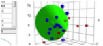
Perfection is defined as all Inside
solvents (Blue solid circles) being within the radius and all Outside solvents
(Red solid squares) outside the radius. Any Inside solvents outside the radius
(or Outside ones within) reduce the Fitness parameter depending on how far
outside (inside) they are. Such "wrong" solvents are marked with a
"*" in the listing and as Blue open circles (for Inside ones outside)
and Red open squares (for Outside ones inside) in the plots.
If you prefer your Sphere to be a wire
frame rather than solid, select the WF option.
Obviously it makes no sense to try to
calculate a Sphere if all your solvents are “Inside” as the program has no way
of knowing the outer limit of your Sphere. Similarly it makes no sense if all
your solvents are “Outside”. The program checks for each of these cases and
gives you a warning.
The analysis of the fit tells you the
number of Inside and Outside solvents (and the total number) the D,P,H and R,
plus the goodness of the fit then a list of the Wrong In and Wrong Out solvents
so you can quickly identify whether their absence of fit is experimental error
or a genuine puzzle.
The data list adds a value for the RED (Relative Energy Difference) number defined by Dr Hansen as
HSP distance between the given solvent and the reference value, divided by the
radius that defines goodness. An Inside solvent has a RED number <=1. A
“Wrong Out” solvent is a solvent that should be Inside but has a RED number
>1. An Outside solvent has a RED number >1. A “Wrong In” solvent is a
solvent that should be Outside but has a RED number <=1.
Some users prefer to grade the Inside and
Outside from 1 to 6 with 1 being Very Much Inside and 6 being Very Much
Outside. If you choose this system then your fit depends on whether you include
the 2’s or the 3’s (or 4’s or 5’s) as “Inside”. You can play with this by
choosing a value from the “Inside” combo-box.
You can also choose a Graded option from the “Inside” choice. If you do this then solvents
with a score greater than 1 are penalised if they are inside the calculated
sphere, but those with a value of 2 are penalised much less for being inside, the 3 are penalised less, the 4’s
are penalised normally and the 5 and 6 values are penalised with increasing
severity. If you have Graded selected when you simply have 0’s for the
“outside” solvents the behaviour is the same as if you had the standard “1”
selected.
How good is the fit? If the data are good
then there is mathematically only one good solution and however often you click
the Calculate button, you will get (nearly) the same answer. If the data are
bad (or if there are too few data points to define a good Sphere) then there
isn’t a unique good fit. The program deliberately starts its search from a
different point in HSP space and if the space is bad, the optimum will be
different each time. So it is always a good idea to click Calculate a few
times. If the calculated values change a lot then you have a broad optimum
which is hard to find. This means either that the sample you are testing is
very inhomogeneous (impurities, co-polymers…), that you have some errors in
your data or that you’ve used too few solvents to define the Sphere
unambiguously.
Another way to evaluate the fit is to look
at the Core values shown in the outputs.
Around the best fit is an area where the
fit is almost as good. The question is, how wide is that area. If it is small
then the fit is very precise. If it is large (maybe just in one dimension) then
the data are not good enough to provide a high-quality fit. The Core values
represent the ± values for the three parameters around the best fit which are
considered “close” to the best fit. The definition of “close” has been chosen
on the basis of tests on a variety of good and bad fits and seems to be a
reasonable indicator that can show good fits (e.g. ±0.25 in all three
parameters) and bad fits (±0.75 in at least on parameter). If the fit is bad in
one parameter that probably means that the suite of test solvents did not cover
a wide-enough range in that parameter.
When you are exploring data you sometimes
get a very large radius which seems improbable to you. You can force the fit to
not exceed the value you include in the Double-click
radius
(see below for an explanation of this value) by checking the Limit box below the double-click radius input.
If you accidentally leave this on you
might get some funny results later on, so use this trick with some caution.
Further Genetic Algorithm (GA) fitting options are described below
What list of solvents do you use? You can
start with ~1200 solvents provided as the default (you can load this at any
time with Open Master Data Set) or the 88 original
Hansen solvents (provided as a reference and also as part of the exhaustive
33/88 file set of all 33 polymers tested with the 88 solvents as in Appendix 3
of the second edition of the Hansen handbook), or a modest Hansen set or you
can create one of your own.
Open
Master Data Set
33 polymers
Files are saved as simple text files
labelled as .HSD (HSPiP Solvent Data). If you want to create a standard set
from a larger set then place a 0 or 1 in the relevant solvents (to show that
they are being Used) and click File
Save Used Only
and only those solvents will be included in the .HSD file saved.
To see just the Used solvents, click the Hide Unused option.
If you over-write an existing file, a
backup is automatically made.
If you’ve loaded a file and want to get
rid of the scores in the column, the Clear button sets them all to
a neutral “-“, preceded by a warning.
If you often want to do this and don’t
like the warning, then Shift-Clear just clears it. If you want them all to be
cleared to “0” then press Ctrl-Clear (with a warning) or Ctrl-Shift-Clear (no
warning).
There are 4 options for opening files:
Open simply opens a file.
Open with Merge merges your chosen file with the current
file. It checks if the number or name is the same as a current entry and if it
is it then checks the HSP and MVol values. If they are all identical then this
entry in the dataset is ignored because it’s already in the dataset. If there
is difference in one or more of the values then the data are added as a row
with a light blue color. At the end of the merge the table is automatically
sorted by name and you can then look for all light blue entries which should be
next to their equivalents. You then have to decide which is the correct value –
knowing that the non-coloured row was the original in the table. Once you’ve
decided on the correct row, simply highlight the bad row and press Delete to
remove it. Remember to save the merged file when you’ve done all the
corrections.
Open with AutoCheck checks each entry and if it matches the
name and number of the entry in the Master Data Set its HSP are automatically
updated to that in the dataset. You should do this for critical datasets each
time there’s a major revision of the HSPiP program with, therefore, some
changes in some of the values. The number of changes is usually very small and
the chances that you have older values is even smaller, but it’s worth doing if
you want to be absolutely sure. The checking can be a bit slow, so be patient.
At the end of the checking a message appears to tell you what values (if any)
were changed. Remember to save the revised version if you are happy with the
changes.
Open Master Data Set, as mentioned above, opens the whole
official set if that’s useful for you.
You can sort the list of solvents simply
by clicking on the relevant column. One click will sort that column Descending,
the next click will sort it Ascending. The sorting of the Name column makes an
attempt to conform to intelligent chemical sorting criteria, but you’ll have to
forgive occasional lapses.
To Delete an entry, click on the row
selector at the edge (just as in Excel) and the whole line is selected. Then
press the Del key. You can highlight multiple rows using combinations of
Ctrl-Click and Shift-Click so that you can delete multiple rows with one
action.
To see a plot of all your current
solvents without performing a calculation, click the S Show button.
If you are trying to create your own
solvent set, this Show function is useful as you can see how much of HSP space
your solvents cover and whether you have too many in one area and too few in
another. There is a mixture of art and science in getting a good test set for
your own application. You have to balance precision (the more solvents, well
distributed, the more accurate the values) with speed (the fewer the faster) and
safety/convenience (some solvents in “interesting” locations can be hazardous).
If you know your polymers are rather aromatic, there’s little point in testing
with lots of solvents with high H/P values, and hydrophilic polymers will gain
little insight from a lot of tests with low H/P values.
Note that many users are so used to the P
vs H plot that the D values tend to get neglected. This can be a major error.
Focus as much on the H vs D and P vs D plots as on the P vs H plot.
Improving
your fit
One way to improve the fit is to use the MVC Molar Volume Correction.
This modifies the fitting algorithm so
that bigger good molecules and smaller bad molecules are accepted as “out” and
“in” respectively on the basis that their molar volumes decrease and increase
their solubility respectively. The Sphere that results can show good molecules
outside, but that’s OK if they are small. The relative molar volumes are shown
(exaggerated) as different sized spheres are cubes.
Another way to look at the quality of the
fit is via the “Core” values shown in the output.

This attempts to show how much the centre
of the Sphere can move in the different directions without incurring too high a
penalty. Clearly the larger the Core values, the less tightly the Sphere is
defined, so some extra solvents might be necessary to refine it. This links in
to the SRC option, described next.
How do you know if you’ve used enough
test solvents to really define the Sphere and its Radius? Following a user’s
suggestion we’ve added an interesting technique. By clicking the SRC option before pressing the Calculate button the program
carries out a Sphere Radius Check. It goes through a list of 80+ solvents (based on the
classic 88 solvent list from Charles) and finds any that are near the boundary
of the Sphere (i.e. they have an RED of 0.9 to 1.1). It then checks each of
those solvents for closeness to solvents in your test list. If they are close
then you already have sufficient data in that area. But if none of your
solvents is close then it’s likely that this test solvent would provide useful
new information to help improve the quality of the fit.
Each of these solvents is added to your
current list and a message appears summarising what has happened. These
solvents also appear in orange on the 3 2D and 1 3D plot so you can see which
holes in solvent space they are filling.
What do you now do? You are smarter than
the computer. So you use your own judgement. Are any of these solvents really
providing useful extra information? If so are these solvents
available/safe/convenient? Is it worth doing an extra few solvent checks?
You even have a different judgement to
make. If you think that that part of solvent space would really be useful to
fill, but you don’t like the suggested solvent (or it’s not in the lab) you can
go to Solvent Optimizer to find a solvent blend that would give you something
close.
Finally, you may want to use a different
set of solvents for the SRC. Feel free to open SphereCheckMaster.hsd file and
add/remove solvents via the usual manner.
In other words, don’t click the SRC
option unless you want to get involved in more work and more decisions. If
“good enough” is good enough for your fitting data, then maybe it’s not worth
trying the SRC option. But it might just suggest a relatively easy 1 or 2 extra
tests that would help pin down the Sphere values, so it’s a good idea to at
least have one go with the SRC option.
Genetic
Algorithm Advanced fitting options
If the GA option is selected then
a new window appears offering you a choice of 3 methods:
•
Classic GA. This sets different
criteria for optimal fit and, of course, reaches its optimum via a different
method from the classic Hansen Sphere algorithm. The “Fit” quality is
calculated differently from the classic algorithm and is only intended for
comparison with other GA fits – not for comparison with the classic Hansen fit.
•
Double Sphere. This assumes that your
material (e.g. a di-block co-polymer) is best described with two spheres.
•
Data points. This assumes that your
values are real data such as solubility, where more is better (unless you
select the “Good is small” option).
This fit makes the maximum use of your hard-won data and will generally
be more accurate than any “good/bad” split. The downside is that “Radius”
becomes meaningless so you have to provide your own value for the plot and RED
calculations.
As a check, you can select the Split
High/Low
option and set a value dividing good from bad and then get a Classic GA fit.
You can choose a Use Log Fit option which changes
the numerics and might give a different answer. An alternative way of fitting
to Data points is via Fit to
Exponential.
This has the advantage of showing the results of the fit, either as a plot of
experimental v calculated (Show
Fit)
or as a plot of solubility against distance (Show Distance). The MVC option should be selected if the solubilities are by weight
rather than molarity – but in practice you can try the fits with and without
this option to see which is better.
In all cases the algorithms require an
initial guess. This can be provided automatically from the data. But if you
have reason to believe the true value is in a certain region, you can get the
GA algorithm searching in the right area by providing your own initial guess. If the fitting space is very clean then
the results are independent of the initial guess – the algorithms always reach the right answer. If the space is very complex then
the initial guess might help steer the algorithm into the right area.
The GA algorithms can be slow. You can
choose a trade-off between Accuracy (Lower, Medium, Higher)
and speed (Faster Slower). Use the Lower
setting when you want to explore whether the GA options are relevant and Higher
when you want a definitive final value. Medium will be adequate for most
purposes if you want a single setting.
Those who require even more options
(including “elliptical” or “variable coefficient” fits) can use the Y-Fit Power Tool.
To close the Advanced options de-select
the GA option.
Adding
solvents to your list
It often happens that you have a list of
solvents and want to add another. It would be very inconvenient to have to look
up the HSP of the new solvent and to type them into your list. If you click the
Master List option then the 3D
diagram is replaced by the master list of solvents supplied with HSPiP. (You
can see the “official” list or, by checking 10K, the entire database of
10,000 molecules). If you double
click (or Alt-click) on a solvent then the HSP (and MVol) parameters are added
to the end of your solvent file.
To hide the list either de-select Master
List or click any of the calculation buttons. See below for creating your own
Master List
As the solvent list is so long, it is
helpful to be able to use the Search tool to find the solvent you want. When
the master list is visible then Search applies to this list, not to your
current solvent list. As soon as the master list is closed then Search applies
to your current solvent list.
If your list is the Master Dataset then
you can also search by CAS number and formula. The search also checks for
alternative names. For example a search for Hydroquinone (which is not a name
shown in the Master Dataset) finds 1,4-Dihydroxybenzene (1,4-Benzenediol).
Starting
a whole new set of solvents
If you already have a reasonable list of
solvents then adding/deleting a few for a different experiment is simple. But
if you have a very different set of solvents, it’s often easier to do File New (or Ctrl-N) and start with an empty
table. Creating a fresh solvent list using the trick in the previous paragraph
(the Master list is automatically opened) is quick and efficient.
Copying/Pasting
HSP
The more you use Sphere, the more you
find yourself wanting to transfer HSP values from one part of the program to
another. Wherever it makes sense, if you click on some HSP (within a table or
within a set of 3 HSP values) and click Ctrl-D (for Duplicate) and Ctrl-P (for Paste) you can transfer the HSP values and, where relevant,
the Molar Volume as well. It’s far easier than having to type them in from
memory! We use Ctrl-D and Ctrl-P because you
might want to use the conventional Ctrl-C and Ctrl-V for conventional Copy/Paste
activities.
For copying a Full line of data from the
Master database, use Ctrl-F.
Graphical
output
The classic HSP plot is Hydrogen Bonding
along the X-axis and Polarity along the Y-axis. When you look at this plot you
often see Outside solvents inside the radius. But of course, HSP space is
3-dimensional. You need to look at the H vs D plot and P vs D plot to get the
full picture. Note that the D-scale in these two plots is expanded by a factor
of 2 as is standard (relating to the factor of 4 in the “Distance”
calculations).
The default setup for the graphics is
that D varies from 10 – 22.5, P, H vary from 0 – 25.
This gives you the classical spherical
plots and covers a good general range. For specialist applications you can
choose to change the D-min down to 0, but always
with a fixed range of 12.5. P-Max and H-Max can be varied over a wide range, always with a minimum of 0
to suit your application. The options may seem somewhat odd, but having tested
the application with numerous data sets covering a wide range of different
applications, this seems the best mix of power and convenience. With different
scale values then, of course, you get non-spherical plots. Remember, the plots
are only a visual aid so don’t get too worried if they are elliptical instead
of spherical. Changing any of these graphical parameters has no effect on the calculations.
If you click the Spherical option the program finds the maximum
scale and sets everything to that to ensure you get a spherical plot. This
might mean that you reduce the visibility of details in the smaller directions
– but you can turn it on or off as you wish.
When you move your mouse over the plots
you get the appropriate parameters and, if close to a solvent, the name.
A 3D plot gives you a global overview.
The colour/shape scheme in the 3D plot is matched to that of the 2D plots. You
can click and drag the mouse to change the orientation of the plot. As elements
move behind or in front of other elements their colours change to give a
further idea of the 3D dimensionality. It will take some exploration before you
are confident of what you are seeing in the 3D view. If you press the Shift key
whilst doing this then moving the mouse zooms the 3D view.
If you press the Ctrl key whilst moving
the mouse then you can pan the graph left/right and up/down. Just experiment
with a plot and you’ll quickly work out how to move around in 3 dimensions.
Anytime you want to bring the 3D view
back to normal, click the little X button below the 3D
graph.
If the size of the form is changed, the
3D view is kept to its original aspect ratio (width/height) to avoid 3D
distortions. This means, for example, that if the form is stretched only in the
width direction, although the 3D box expands to fill the width, the 3D view
expands rather less so that if you pan the 3D image it gets cut off towards the
right hand side.
So, for a larger 3D view make sure you
expand both width and height.
Sometimes you want to see just the Inside
solvents, sometimes just the Outside. And sometimes it’s useful to have a label
on each 3D element to tell you where your solvent is – the label can be either
the number (less cluttered) or the name (more cluttered but more direct). You
can choose from each of the 9 possible options to get the view that is most
helpful to you.
And you can choose a 10th
option – the minimum sphere that encloses all the Inside solvents. This is
handy when you are checking for a property (such as reactivity) where being
inside is necessary but not sufficient. In other words, many chemicals might be
inside the sphere but don’t (e.g. for functionality reasons) react with the
target. So a classic Sphere calculation tries to minimize the number of these
“wrong in” compounds, even though they aren’t strictly “wrong”.
Finally the 11th option, “Data
only” shows just the data points without the sphere.
Identifying
individual solvents
Moving the mouse over the 3D plot shows
the name of the solvent.

Identifying a 3D element from a 2D screen
is a somewhat complex task so the response can be somewhat slow if there are a
lot of solvents. For the full data set the technique isn’t 100% reliable so
some solvents come out as “Unidentified”.
To see a few solvents more clearly, if
you select one or more solvents by clicking on the left-hand edge so that the
whole line is highlighted, and then click the SSel (Show Selected) option
then when you plot the Sphere, the solvent(s) will be shown in orange in the 2D
and 3D plots. If you select either the Name or No. option then only the name
(or number) of the selected solvent(s) will be shown in the 2D and 3D plots. This
trick can sometimes be useful for identifying interesting features in your
data.
Finding
a solvent in the list
If you have a long solvent list, it can
be tricky to find a particular solvent as you might have a different naming
convention from that in the list. If you know the standard Hansen number for a
solvent (e.g. 325 for Ethanol) simply type the number into the search box and
press Enter or click the Find button. If you want to find all solvents
containing the fragment “pyrrol” then the table will show only those chemicals.
The less you type (“pyr”) the more chemicals will appear in the table.
The searches are case insensitive so
PYRROL, Pyrrol and pyrrol will each find the same entries in the list.
Note
that chemicals are automatically put into “proper case” when the file is
loaded. This avoids the user and/or the author from having to fuss about
whether to enter ethyl acetate or Ethyl acetate or Ethyl Acetate. Whatever you
enter, next time the file is loaded it will come out as Ethyl Acetate. The
exception is small names such as GBL (Gamma Butyrolactone) which remain exactly
as entered. Of course the program tries (and usually succeeds) to make sense of
entries such as n-butyl acetate which comes out as n-Butyl Acetate and
n-methyl-2-pyrrolidone which comes out as N-Methyl-2-Pyrrolidone. Please
forgive the occasional glitch.
You can also search by CAS number.
To restore the whole list, click the X button.
The
Double-Click method
If you know of a solvent that has a good
HSP set, you might want to find solvents that are within a close HSP Radius of
that solvent (e.g. to find a cheaper or safer alternative to your current
solvent). To do this, simply Double-Click (or, if you prefer,
Alt-Click) on your solvent, having previously entered a Double-Click Radius. The solvents are then
automatically sorted by RED number with your chosen solvent, by definition,
having a RED number of 0. Any solvent with a RED number of <=1 (i.e. up to
your Double-Click Radius) satisfies your criterion and is shown in solid Blue
in the graphs. All others are shown as hollow Blue. If you have too many
“Inside” solvents, reduce the Double-Click R and try again.
If you have a target HSP that is not
included in the solvent list, go to the bottom of the table and enter a D, P, H
set in that empty row. You can add a Number and Name if you wish, but if you
don’t they will automatically be assigned “0” and “Target” when you
Double-Click.
Diluents
in your test samples
Sometimes a polymer or pigment comes with
X% of solvent which cannot be removed before doing the Sphere test. If the
sample is tested as Y% in the solvent (e.g. a polymer might be tested as
soluble/insoluble at 5%) then the HSP of the test solvent is diluted by a
certain %. For example, if the polymer’s solvent is 50% then to have 5% of
polymer you also have 5% of that solvent in the test vial.
To correct for this, you add an extra
line to your .hsd file, with the solvent named as Diluent or Dilutor or
Dilution (whichever makes more sense to you – it must start with DILU), in the
HSP columns you enter the known value of that solvent, and in the Score column
you enter the final % of that solvent. The Sphere fitting automatically adjusts
the HSP of the overall test solvent (based on the weighted average of their HSP
– just as in Solvent Optimizer). Usually the effects are small, but the feature
is added for those who think it might be a problem for their particular case.
ESC
Alert
Environmental Stress Cracking (ESC) is a
complex but important subject involving the interaction of (bad) solvents,
stress and the polymer. When the ESC
alert
option is selected the solvents are colour coded depending on their tendency to
cause ESC. This Help file isn’t the appropriate place to discuss what the
colour coding means, so please refer to the ESC chapter in the eBook.
Solvent
mixtures as “solvents”
Sometimes you need a “solvent” with a
specific HSP for testing the Sphere but can’t find a suitable single solvent.
You therefore need to make a mixture with the desired values. To make this easy
to do, the “S” button in the Solvent Optimizer transfers the HSP value of
whatever mix you have created in the Optimizer over to a new line in the Sphere
solvent table.

Your
own Master List
The master list is encoded within the
software and can’t be altered. This is for many reasons, one being certainty
that whenever any user refers to the master list they are always referring to
the same version.
However, some users want to use their own
master list. Here’s how to do it. First create a .hsd file using any relevant
technique – including doing a large batch conversion process via the Y-MB DIY.
Load it as normal to check that it’s OK. Now save it to the HSPiP Data folder
as MyMasterData.hsd. If you now select MyDB that will now be your master data for all relevant
activities including FindMols and the Y-MB DIY Analog search. As it’s possible for you to have subtle errors in this set,
if the software finds any problems with it, it reverts to the standard master.
You’ll have to find the cause of your problem yourself – typically it will be
some illegal value in one of the key propertie.
If you want to revert to the standard
master, simply un-select the MyDB option. If you want multiple masters, name
them something like MyMasterData1, MyMasterData2… then load whichever one you
wish to use as the master and save it as MyMasterData.
Optimizing
If you want to find a pair of solvents or
a complex mixture of solvents to match a particular HSP then you can use the O Optimize button which brings up the Solvent Optimizer form, with the target solvent
automatically set to the solvent you have currently selected.
To transfer solvents from this form to
the Solvent Optimizer, select one or more solvents by clicking (or
Shift-clicking or Ctrl-clicking, as per any Microsoft-style table) on the
“selection” box on the left-hand edge of each solvent, then Ctrl-Click (or
Right-Click) on the text of one of the selected lines and, after a message
appears for you to confirm that this is what you want to do, the solvents will
be added. This isn’t the easiest of things to get right first time, but Ctrl
and Shift are used for many things by Microsoft and we’ve done the best we can.
Polymers
For dealing with polymer issues, click
the P Polymer button which opens the
Polymer form.
Do
It Yourself (DIY)
To generate HSP values from your own
chemicals and to investigate a whole range of interesting properties such as
activity coefficients, HSE “read across” and solubilities, click on the δ
button.