2017 is the 50th anniversary of the Hansen solubility parameter. The anniversary lecture was held in York, UK, where I gave two keynote talks.
The highlight was Hansen-Hiroshi-Steven Solubility Parameters for Prediction, HHSSPP= HSP2. It is my hope that it will be used for 2500 years, the square of the 50 years.
I thought of many new names.
For example, Expanded HSP.
But with EHSP, you won’t be able to find it on the Internet.
English for High School Preparation
Enhanced High Speed Processor
Equine Health Studies Program
It’s not a good idea to put anything in front of it.
Keep brand identity of “HSP”
Network searchable.
Image of new and powerfulness.
So I decided HSP2.
At the same, 50th anniversary lecture, Dr. Lerche from Germany was using HSP for dispersion, especially for inorganic materials. He said that inorganic materials do not “dissolve”, so this is “dispersion”, and therefore Hansen Dispersion Parameters (HDP) is correct.
I found web page made by a Japanese company called MS Scientific, Inc.
They had started their evaluation service using Dr. Lerche’s LUMiSizer, a dispersibility evaluation and particle size distribution measurement instrument
In their Web page, they write:
The Hansen Dispersibility Parameter (HDP) is an indicator of the affinity and dispersibility of fine particles and nanoparticles to a solvent. It predicts the solubility and dispersibility in various solvents and is widely used in various scientific fields such as the coating industry and surface science. The Hansen parameter is a property evaluation method that has attracted particular attention because it can be used to select and design appropriate dispersing solvents for slurry production.
But since neither HSP nor the letters Hansen Solubility Parameters were used, my search so far did not turn up any results.
So, let me advertise them a little.
Their device, the LUMiSizer, is a very good device for evaluating the dispersion of inorganic materials. This time, I was able to get some data that can be obtained by using their device, so I did some analysis.
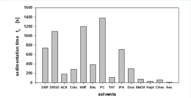
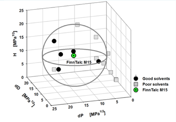
With this device, for example, we can get the Sedimentation time from a pigment dispersed in 14 different solvents. In some solvents, it settles quickly, but in others, it settles slowly. Then, we turn it into Relative Sedimentation Time (RST) (how?). If you do HSPiP analysis with RST norm >0.5 as good solvent and <0.5 as poor solvent, you can get HSP of pigment and Hansen Solubility Sphere.
This is the standard way of using HSP so far, and I’m not saying that what it says is wrong.
But HSP2 will make HSP much richer.
I met Dr. Lerche when he came to Japan and explained this to him, but I don’t think he really understood what I was saying.
For example, ED (Electron Donar) and EA (Electron Acceptor) values of solvents are essential to evaluate the dispersion of basic and acidic pigments. dHacid, dHbase are also important.
In HSP2, dD is also divided into dDvdw and dDfg, so there are 7 different parameters for one solvent.
This calculation method is not yet included in HSPiP, so please copy and paste the data into Excel.
The main problem with such a high number of dimensions is that it cannot be displayed in 3D like Hansen’s dissolving sphere so far.
So, let’s try to compress the dimensions using the Principal Component Analysis (PCA) method.
The PCA method is AX because it transforms the axis (Axis).
Principal Component Analysis (PCA)
Japanese visitors should also refer to pirika’s PCA page.
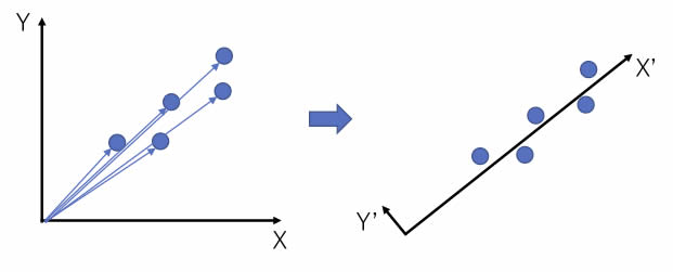
For example, in the figure on the left, there are five two-dimensional vectors.
The size of the vectors are different, but the orientation is very similar.
So, if we rotate the X and Y axes, we get the figure on the right.
The X’ axis is roughly the size of the original vector, and the Y’ axis has a very small value. If the value of Y’ is small enough, the rotation of the axis will reduce the two-dimensional vector to a one-dimensional vector.
In this way, we first take the largest tendency of the vector as the first principal component, and the axis orthogonal to it as the second principal component, and so on.
What seems so simple when written like this, when you decide to try it, you will probably have no idea how to do it.
Don’t worry! In this day and age, if you learn how to set up data, even if you don’t know what it means, you can just click a button and PCA web app will do the calculations for you. Statistics and analysis are highly compatible with AI, so you won’t need a data scientist any time soon.
Learn just how to set data and receive results!
It is hard to analyze 7-dimensional data at once, so let’s choose two columns.
Let’s choose two columns that have a high correlation with the sedimentation rate.
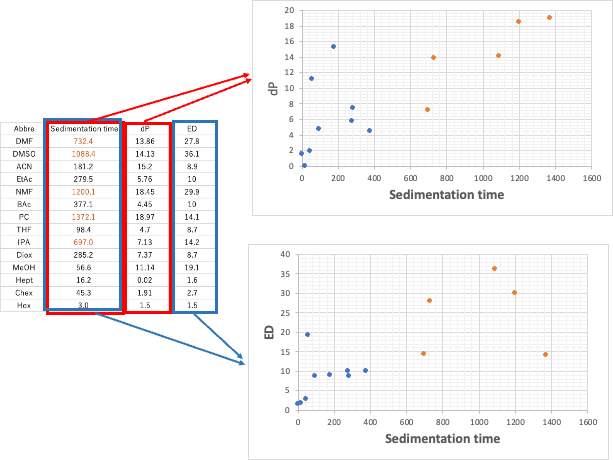
Let’s add a new Tab to the Excel table we just created, and create a table with Abbre in the first column, sedimentation time in the second column, dP in the third column, and ED extracted in the fourth column, and draw a graph. Those with sedimentation rates above 500 are shown in orange.
It is clear from this graph that the sedimentation rate is highly correlated with dP and ED, respectively. There are a few exceptions, but the solvents with large settling velocity have large dP and ED.
So, when we plot dP to ED on a graph, there is a high correlation as shown in the left figure below.
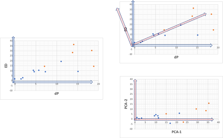
This means that the [dP, ED] vectors representing each point have different magnitudes, but similar orientations. So, we should be able to find the new red axis in the upper right. As shown in the lower right figure, in this case, the second principal component will also have a maximum value of about 15.
It’s hard to explain, but anyway, let’s press the Calculate button.
A new tab will be opened, and if you set Calc.PCA as ReadData, the answer will come back.
From this result, we can see that only 86.98% of the data can be represented by the first principal component alone.
The important thing is the formula of Calculate Scheme. Copy this formula and paste it into the second row of the appropriate column in Excel with the = sign. (The reason for the second line is that the formula refers to columns C and D of the second line.) This will be the X coordinate of the new axis.
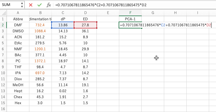
Paste the second equation in the same way. This will be the Y-coordinate of the new axis. If you plot this, you will get the figure on the bottom right.
Once we know this, we can apply it to the 7-dimensional data. If we take into account the third principal component, we can express up to 92% of the data.
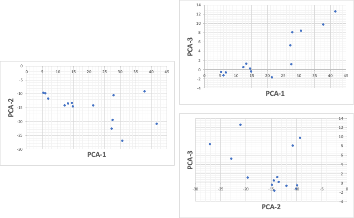
However, it would be impossible to construct a 3D position in our brain from these three graphs.
Let’s use plotly.js, a graphing software, to display them in three dimensions.
This will be the new Hansen space in HSP2.
If we find a Hansen2 solvation sphere that contains all the solvents in orange inside the sphere, we can predict that all the solvents that go inside the sphere will have a sedimentation rate of 500 or higher.
If you want to do a more quantitative analysis, you can use the GROVE analysis tool that we created.
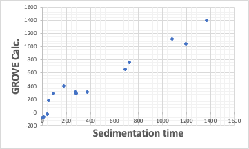
Select three important variables from the seven variables of HSP2 to create a prediction equation for sedimentation rate.
sedimentation rate=-173.54*dHAcid+13.23*ED+75.12*EA+-109.98
If four variables are selected, then dDvdw is selected further.
This means that the sedimentation rate of this pigment is highly dependent on dHAcid (hydrogen bond acidic term), ED (electron donor), and EA (electron acceptor).
It is important to remember that if you ignore this and predict from the old 3D HSP only, the “solvents that increase dispersion further” may be less important.
As machine translation becomes more advanced, I’m sure Dr. Lerche will understand what I’m trying to say.
pirika’s DX aims to enrich interpretation in this way.