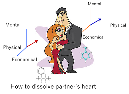
I don’t need to explain that distance is important to dissolve, whether it’s medicine or heart.
The problem is that the degree of importance varies from axis to axis.
Even if the other two are in agreement, the other one may be many times more important.
Hansen solubility parameters are calculated by taking [δD, δP, δH] as vectors and calculating the distances in Hansen space.
The reason why I said “Hansen space” is because it is not a Euclidean space.
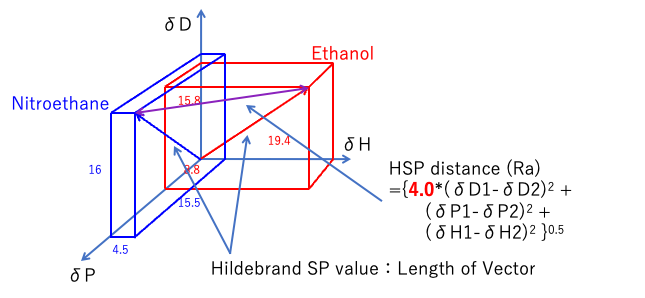
The dispersion term (δD) of the HSP distance is preceded by a factor of 4.0.
So, in Hansen space, if we don’t stretch it twice as far as the δD axis, Hansen’s dissolving sphere will become a rugby ball instead of a sphere.
This was also said that HSP is very useful in practice, but theoretically meaningless because it contains the incomprehensible parameter 4.0.
For this problem, I showed that it can be solved by using the new HSP2 in the 2017 HSP50th anniversary, memorial lecture. It will be an important point in HSPiP ver.6 which will be announced soon, so I will dare to explain it.
Hansen Solubility Parameters, Discussion of Dispersion Term (δD)
No one would disagree that noble gases have very weak intermolecular forces.
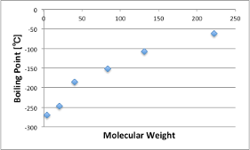
Let’s look at the relationship between their molecular weight and boiling point.
Helium, Neon, Argon… The higher the molecular weight, the higher the boiling point.
If I add the molecular weight and boiling point of the perfluorinated and perfluoroether compounds to that, I can see that they also ride the same curve.
This means that the compounds have a base intermolecular force that depends only on the molecular weight (molecular volume).
It will be a weak VDW force, which molecule will always have if molecule have the molecular weight.
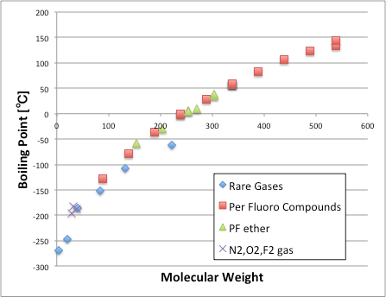
Based on this result, PTFE, a fluoropolymer, can be considered as a polymer of noble gases (with no intermolecular interactions with other substances).
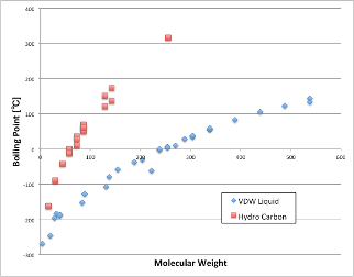
If you plot the chain hydrocarbons there, you will see the red square.
According to Hansen’s theory of solubility parameters, chain hydrocarbons have only δD (dispersion term), and δP and δH are zero.
However, the δD (dispersion term) of hydrocarbons has even larger intermolecular forces than the weak VDW forces due to the molecular weight of noble gases. (So, higher temperatures are needed to break that force.)
The defining equation of solubility parameter is as follows。
δ=((Hv – RT)/Volume)0.5 Hv: Heat of Vaporization
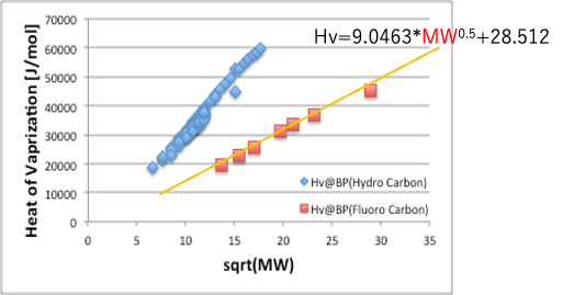
Trouton’s rule says that the latent heat of evaporation at the boiling point divided by the boiling point is constant in a regular solution. So, let’s try axis conversion.
If we take Hv as the vertical axis and the root of molecular weight as the horizontal axis, the curve of fluorine compounds becomes a straight line.
So, the Hv of the base part is ,
Therefore, the Hv of the base part can be expressed as 9.0463*MW0.5+28.512.
If we take the root of the latent heat of evaporation divided by the molecular volume, we can get the solubility parameter corresponding to the weak VDW.
We define it as δDvdw.
δDvdw=((9.0463*MW0.5+28.512)/(MVol))0.5
For any molecule, the molecular weight (MW) is easy to get and the molecular volume (MVol) is easy to calculate with Y-MB.
In addition to the δDvdw, hydrocarbons are considered to have intermolecular forces that depend on the functional groups of the molecule. The solubility parameter for this is defined as δDfg.
δD2 = δDvdw2 + δDfg2
δD is the original HSP, so we have the data. Since δDvdw is easy to calculate, δDfg is also easy to find.。
In HSP50, I proposed the following equation for distance.
Distance1967={4.0*(δD1-δD2)2 +(δP1-δP2)2 +(δH1-δH2)2}0.5
Distance2017 = {(δDvdw1-δDvdw2)2 +(δDfg1-δDfg2)2 +(δP1-δP2)2 +(δH1-δH2)2}0.5
Gone is the 4.0, and in its place is the 4-dimensional Euclidean distance.
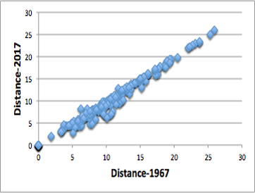
Using this new distance, I tried to apply it to the solubility data of polymers in HSPiP.
The formula proposed by Dr. Hansen in 1967 requires a magic number of 4.0, and all distances between polymer 88 solvents were calculated.
Comparing the distances calculated by the formula with the distances calculated by the new formula, a very high correlation was observed as shown in the figure on the right.
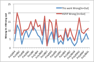
Using this distance equation, I checked the number of good solvents that went out of Hansen’s sphere by mistake and the number of poor solvents that went into Hansen’s sphere by mistake when I analyzed the example, and found that all the systems improved.
From this result, there is only one reason not to split δD and use the new distance formula.
In other words, there was no way to visually represent the 4D data.
In this regard, I have posted an example of dimensionality reduction using Principal Component Analysis (PCA) on my blog, so please refer to that as well.
Now that I finally have an idea of how to use this parameter, I’m going to hurry up the development for ver. 6.
By the way, let me introduce the most important result of using this new set.
Both silicone oil and fluorinated oil are very hydrophobic and do not dissolve in water.
They are very hydrophobic and do not dissolve in water, and although their HSPs are very similar, they do not dissolve in each other.
| Name | dD | dP | dH | 1967 Distance |
| Dimethoxydimethylsilane | 12.82 | 3.19 | 4.03 | 2.04 |
| 1,1,2,2,2-Pentafluoroethyl 2,2,3,3,3-pentafluoropropyl ether | 12 | 3.59 | 2.88 |
| dDvdw | dDfg | dP | dH | 2017 Distance |
| 9.88 | 8.16 | 3.19 | 4.03 | 8.5 |
| 12 | 0.02 | 3.59 | 2.88 |
However, if you look at the new distance formula, you will see that it is 8.5, which clearly shows why they do not blend together.