Some students participating in the PIRIKA research group are performing optical resolution. While looking for lecture material, I found a paper on optical resolution by controlling the dielectric constant in a mixture of alcohols and water.
The original article “Advances in chiral drug production technology” in Bulletin of Gunma Perth University No 23 – New engineering partitioning technology to control molecular recognition – is available online.
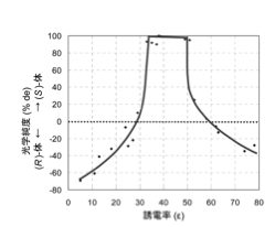
Roughly speaking, the optical purity of the (S)-body is higher when the dielectric constant is between 30 and 55 (this range depends on the compound), as shown in the diagram above, and the (R)-body is higher otherwise.
I therefore searched for data on the dielectric constant of solvents mixed with alcohols and water.
Although it was an old paper, the value was found in the paper ‘Relationship between the dielectric constant of organic solvent-water mixture solvents and the solubility of electrolytes’ in Chemical Engineering Vol. 28, No. 11 (1964).
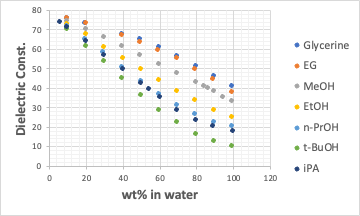
When scanned and summarised, it looked like this.
A QSAR equation is currently being constructed to deduce the dielectric constant from Hansen’s solubility parameter for another application. Originally, the δP term (polarisation term) of the Hansen solubility parameter was determined from the dielectric constant.
The HSP of a solvent mixture can be easily calculated using the volume fractions (φ1, φ2) as follows.
HSPmix = HSP1φ1 + HSP2φ2
(However, water/alcohol may cause azeotropy, so the activity coefficient may also have to be taken into account).
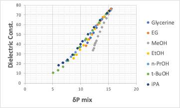
Therefore, the horizontal axis in the above figure was changed from weight % of the mixture solvent to tot HSP(= sqrt(δD2+δP2+δH2)) of the mixture .
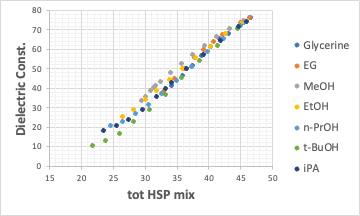
It was then found that the dielectric constant and tot HSP have an almost clean linear relationship.
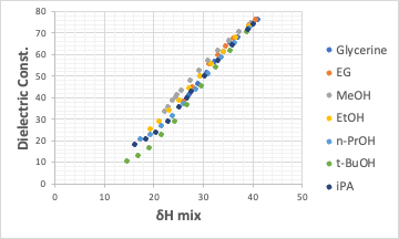
Its seems that the essence of the correlated tot HSP is δH and not δP.
If a linear relationship can be obtained between the solubility parameter and the dielectric constant in this way, it means that the abscissa of the first figure can be plotted as tot HSP or δH.
And if HSP is used, the solvent mixture can be calculated as a volume fraction. So a mixture with the required HSP (which changes rapidly in a fairly narrow range) can easily be designed using HSPiP.
Apart from alcohols, acetone and dioxane deviate slightly from the alcohol line.
This means that donor/acceptor properties may be in play.
Let’s dig a little deeper into that with the students.
Well, we can write as many papers as we want.