2025.7.20
pirika.comで化学
>チャピエモン-3rd Pirika Origin (CPO)
> ハンセン溶解度パラメータ (HSP)
>HSPiP(実践ハンセン溶解度パラメータ)ソフトウエアー
> HSPiPの購入方法
> HSPiPを用いた解析例
>次世代HSP2技術
> 化学全般
>Pirika ツール群
ブログ
業務案内
お問い合わせ
注意:HSPiPの機能ではありません
私のブログには電子ビームレジストポリマーのGs(100 eVあたりの主鎖切断数)の予測についても書いている。現像液の設計については、「QSphere: 定量問題の解決」で説明した。
溶かさない溶媒設計ーレジスト現像液 2026.6.20
半導体用レジストポリマーの現像液設計(非溶媒設計)に関するv-tube動画もある。
横浜国大での講義資料だ。。
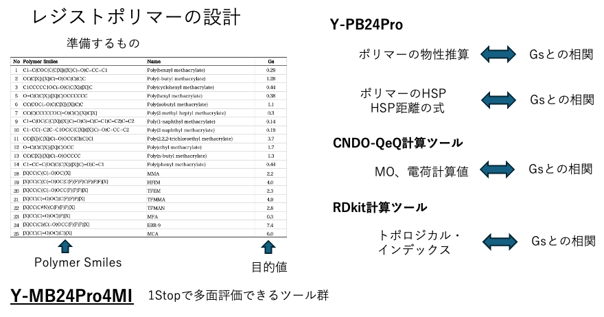
次のようなポリマーがあるとき、100 eVの電子ビームで何個の結合が切断されるかを予測する式を作ってみよう。これは2011年の授業で話した内容だ。
electron beam resist polymer

赤で示した企業は、横浜国立大学の学生が就職している企業だ。将来、そのような企業で働き、レジストポリマーを設計する場合、どのようなスキルを身につけておくと役立つだろうか?
今回はエステルに限定し、『Polymer Handbook』から追加してポリマーを分析してみる。各ポリマーのSmiles構造を用意した。分子描画ソフトJSMEを使ったSmiles構造の取得方法についてはこちらを参照してほしい。
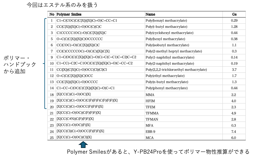
準備が完了したら、あとはPirikaProにjobを放り込むだけだ。PirikaProはWebアプリのスタンドアロン版(EXE)だ。Mac、Windows、Linuxで利用可能だ。YPB-24を選択する。
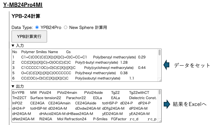
Data TypeとしてYPB24Proを選択する。Polymer Smilesで作成した4列を入力欄に貼り付け、Calc,ボタンを押す。各Polymer Smilesを解析し、ハンセン溶解度パラメータ(HSP)を含む様々な熱物性値を推算する。これらの熱物性値を用いてMIを計算する。
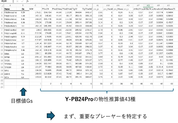
1列目はポリマーの名前など、目的変数(教師データ)は2列目に記載する。ここでは2列目がGsだ。そこへ説明変数43個を追加した表が即座に作成できる。
完成後、まずmajor playerを特定する。
PirikaProで拡張相関係数計算ツールを選択する。
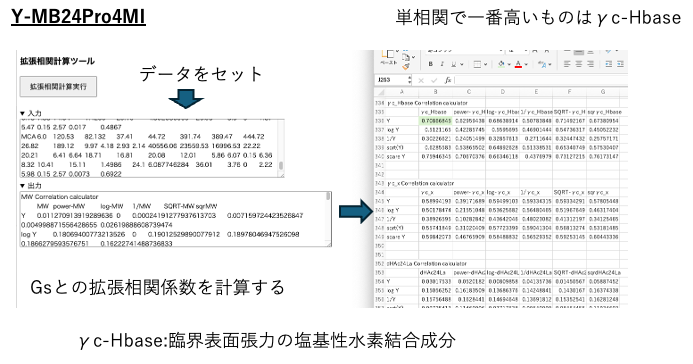
これはGsと43個の説明変数間の単純相関を計算する。その際、変数の対数や1/X、√Xなどの計算もふくめ相関係数を出力する。最高相関係数を示したのはγc-Hbase:臨界表面張力の水素結合塩基成分であった。Y-PB24Proでは、臨界表面張力(γc)をHSPと同様に分散項(γcd)、分極項(γcp)、水素結合項(γch)に分解する。この水素結合項はさらに酸性成分と塩基性成分に分割される。接触角の推算を可能とする新規追加の物性値である。
主要因子が特定されたら、次のステップは重相関を検証することだ。
PirikaProで変数選択重回帰法を選択する。
V-tubeを作った
読むより見る方が楽だろう
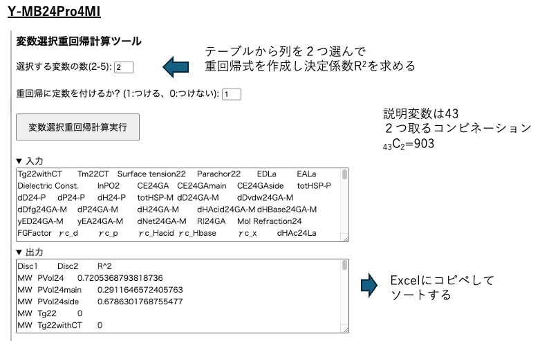
説明変数は43個あるため、2列を選択すると43C2、つまり903通りの組み合わせが生じる。これら全903通りの組み合わせに対して重回帰分析を実施し、決定係数(R²)と共に結果を出力する。結果はソートされていないため、Excelに戻して降順で並べ替える。
同様に、3つの変数を選択し変数選択重回帰分析を実行する。列数は最大5つまで選択可能だが、CPU性能やメモリ容量によっては大幅な時間を要する可能性がある。2~3列の選択が適切と考えられる。
R²の降順で並べ替えることで、Gsの大きさを記述するためにどの列を選択すべきかを定量的に把握できる。
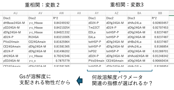
3つの変数を選択する際、溶解度パラメータに関連する変数が頻繁に選ばれる。これはGsが溶解度パラメータに支配されていることを示している。一見すると意外に思えるかもしれない。HSPはレジストポリマー開発における溶媒選択で広く用いられている。しかし、電子ビームを用いて結合を切断するプロセスにおいて、溶解度パラメータはどのように影響するのだろうか?
そこで、YMB24Pro4MIで多重回帰分析を選択し、まずGsの文献値と多重回帰計算から得られた値を比較した。
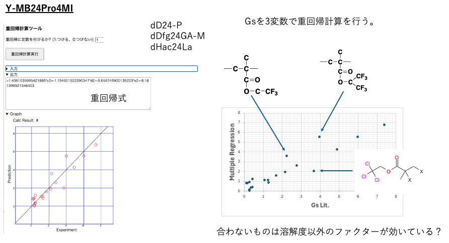
3つのハロゲン系ポリマーが著しく逸脱している。これは溶解度パラメータ以外の要因による可能性がある。しかし、残りのポリマーは溶解度パラメータによって非常に良く説明できる。
溶解度パラメータは以下の式を用いて評価できる。
SP=(凝集エネルギー/単位体積)0.5
推算された凝集エネルギー値をY-PB24Proが出力する物理特性値のGsと比較する。大きく乖離する値が3つ存在するため、単一の相関は高くないが、その他の値にはかなり明確な相関が認められる。
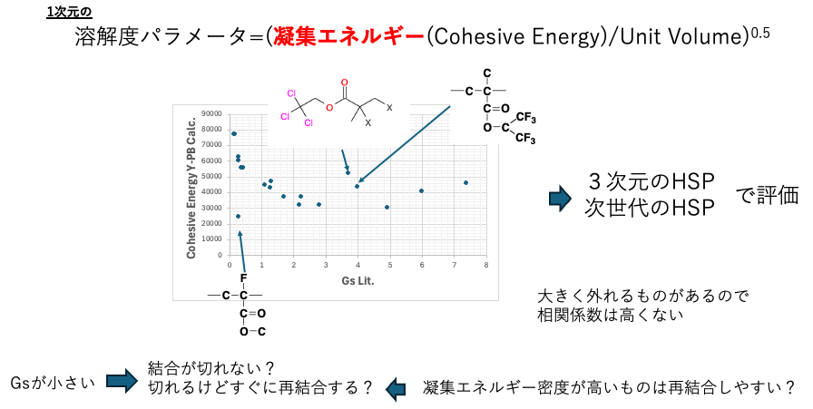
凝集エネルギーとGsの間にこのような相関関係が存在する事実は、凝集エネルギーの高いポリマーは電子ビームによって切断できないか、切断されても速やかに再結合することを示唆している。この場合、SP値は一次元的なSP値となる。我々は三次元(n次元)ハンセン溶解度パラメータを用いてこれを評価する。
次世代HSP向けSphere計算のデータ形式を作成するには、YPB24Proで「New Sphere計算用」ラジオボタンを選択し、計算を実行する。
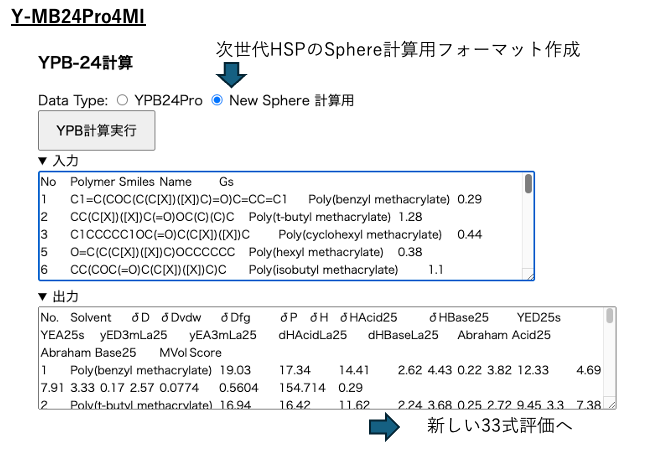
取得した出力をExcelに返す。
33式を用いた新たな距離計算ツールはPirikaProに含まれると説明されているが、実際には別のプログラムである。これは計算負荷が非常に高く時間がかかるため分離された。速度最適化のため並列計算を実行するWorkerが使用される。
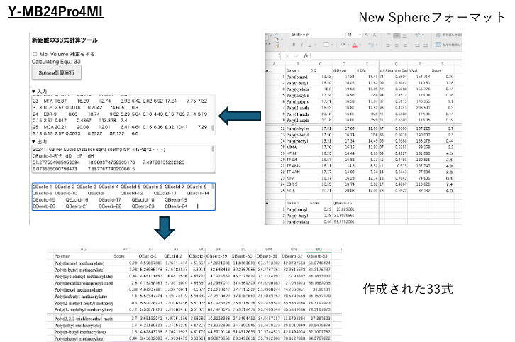
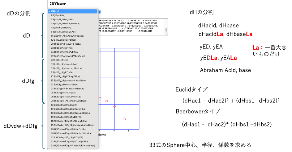
新しいSphereフォーマットのデータを33式計算ツールに貼り付け、計算を実行する。計算が完了するまで約5分間待つ。HSP距離の33式の詳細については、こちらの資料を参照してほしい。
待っている間に、ハンセン溶解度パラメータ(HSP)距離を確認する。
HSPは3次元ベクトルとして表現される。3次元空間にプロットすることで空間上の位置が明らかになる。ハンセンが開発したSphere法でハンセンの溶解球を探索する。球の中心が決まる。球の中心とベクトルの終点との距離をHSP距離と呼ぶ。当然ながら、4次元以上の空間では球とは呼べない。定義は式の「内側」または「外側」となる。
Sphere法の基本
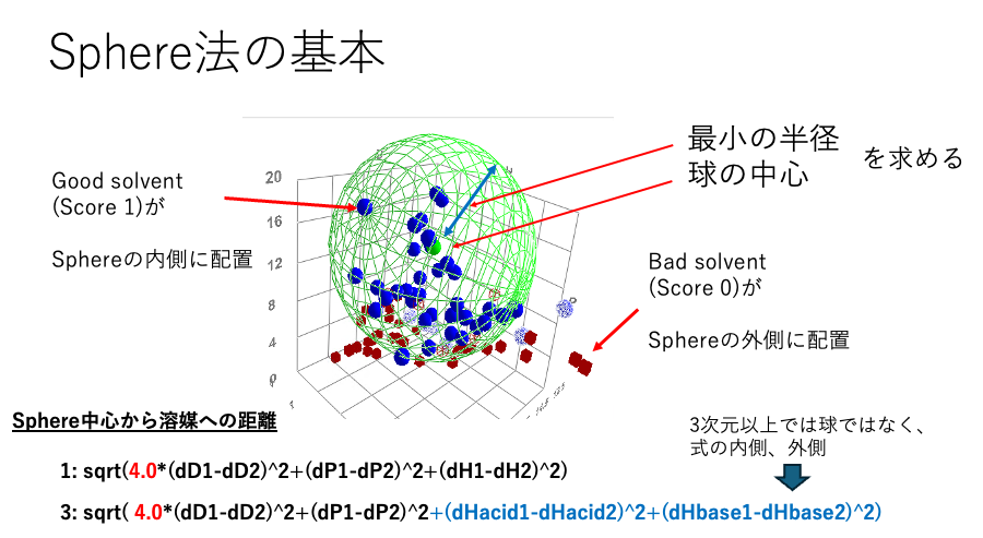
この球の中心からのベクトル距離と物理的特性との間には、明確な相関関係が存在する可能性がある。
類似したHSPベクトル(空間内で類似した位置にあるもの)は、類似した特性を持つ可能性がある。そしてそれらの特性は、中心からのスカラー距離が増加するにつれて弱まる。
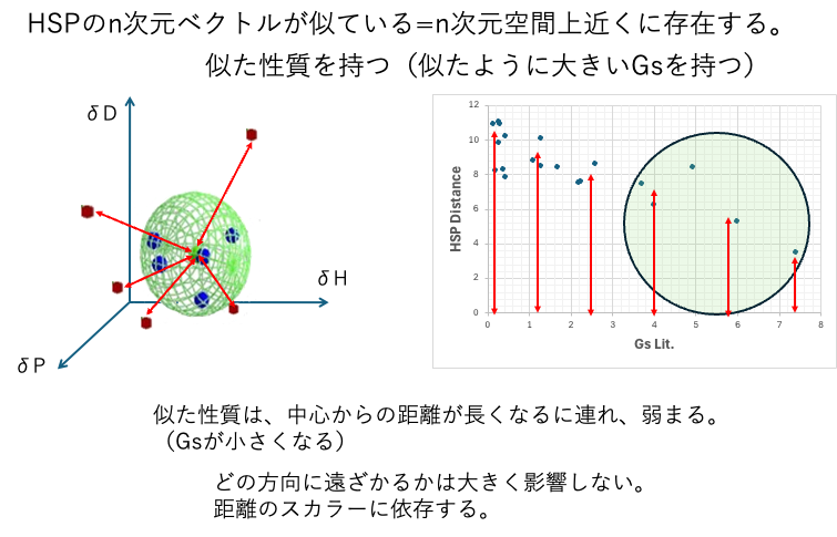
(仮説だが)n次元空間において、似ているn次元ベクトルは似ているG値を持つ。
例えばポリマーが溶解する際、良溶媒が集合して球状を形成することがある。ただし「良」か「悪」かは研究者次第である。時に不都合なものが集合することもある。
私(山本博志)は2017年にこのsphere法を拡張した。まずdD項を分割した。元のSphere法では距離式においてdDの差の前に4の係数が存在する。この4の熱力学的意味が説明できなかったため、常に批判の対象となっていた。
例えば、希ガスは分子間相互作用がないと考えられる。しかし希ガスにも沸点や蒸発潜熱は存在する。そこで分子サイズを持つ分子には、分子サイズに対応する基本SP値を割り当てる。これをdDvdwと呼ぶ。従来のHSPでは基本値を直鎖炭化水素に設定していた。しかし直鎖炭化水素においても、分子サイズに加えCH₂相互作用が存在する。これらは官能基相互作用と呼ばれdDfgで表される。当初この複合ベクトルはdDであったが、長さが半分になったため係数4が必要となった。dDvdwとdDfgを使用する場合、この係数は不要となる。
2017年の拡張

次に、水素結合項を分割した。従来、dH項はdHdo項とdHac項(プロトン供与体と受容体)に分割されていた。しかし、酸・アルコール・アミンなど活性水素を含む化合物以外のすべてについては、dH項の全てをdHacに割り当てた。カルボン酸、アルコール、アミンは、酸としても塩基としても振る舞うことができるため、両親媒性化合物に分類される。
したがって、dHの分割効果は無視できる程度であった。
2017年のHSP50周年記念講演において、私はブレンステッド酸塩基ではなくルイス酸塩基に基づく指標yEDおよびyEA(山本電子供与体/受容体)を紹介した。
これらの値は分子のSmiles構造式から計算可能である(HSPiPには未収録。PirikaProの独自機能)。
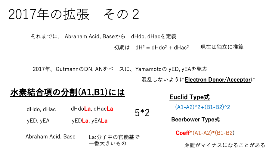
HSPがナノ粒子などの金属を含むシステムで使用されるにつれ、ブレンステッド酸塩基では良好な結果の取得が困難になってきている。HSPは基本的に平均場理論を用いて計算される。この理論では、アルコール分子のサイズが大きくなるにつれて水素結合項は減少する。しかし、分散効果がカルボン酸のpKaに依存する場合、pKaは分子サイズにほぼ独立している(ギ酸を除く)。そこで我々は、分子内で最大のブレンステッド酸/塩基およびルイス酸/塩基官能基のみを考慮する式も導入した。
弱酸または弱塩基の塩に強酸または強塩基を加えると交換反応が起こることが知られている。これを表現するにはユークリッド型式式では不十分であり、場合によってはBeerbowerが提案した式式がより適切である。これら全てを評価すると33式の式式となる。
HSPiPにはタイプ1とタイプ19のアルゴリズムしか搭載されておらず、やや時代遅れだ。
今回はそれらを完全に書き直し、YMB24Pro4MIに組み込み込んだ。
セレクターを確認し、どの式がどの相関に対応するかを確認してほしい。
dDを分割する効果は以下の通りだ。
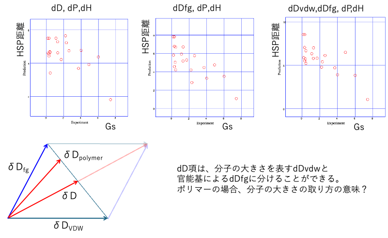
標準的な[dD, dP, dH]において、HSP距離とGSの相関は低い。dDfgとdDvdw,dDfgのどちらを使用すべきかについては意見が分かれるところだろう。
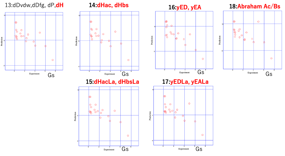
dHの分割に関しては、式16か式15のいずれかが良いだろう。
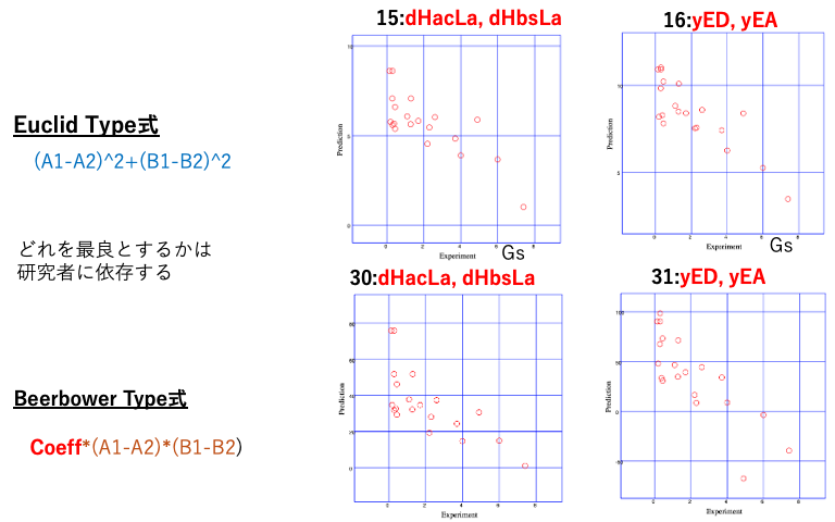
EuclidとBeerbowerのどちらかを選ばなければならないとしたら、難しい決断になるが、おそらく16式を選ぶだろう。
データの作成方法と距離計算式の算出方法の説明
文章で説明するのは難しいので、V-tubeを制作した。
かつて私はKAISTで電子ビームレジストポリマーの設計に関する講演を行った。
その際、多田教授の論文を参照し、分子軌道計算に加えてHSPを用いた解析も適用可能であることを示した。
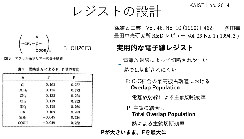
20年後、これを試すのは簡単だ。
YMB24Pro4MIツールでCNDO-QeQ計算ツールを選択する。
ポリマーSmiles内の[X]を[H]に置き換え、計算を実行する。
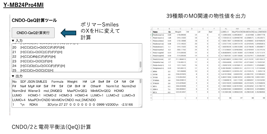
39種類のMO関連物理特性値が取得できる。
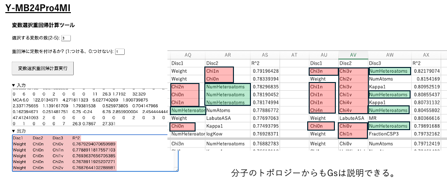
この表を用いて変数選択重回帰分析を実行する。
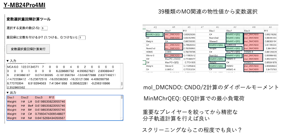
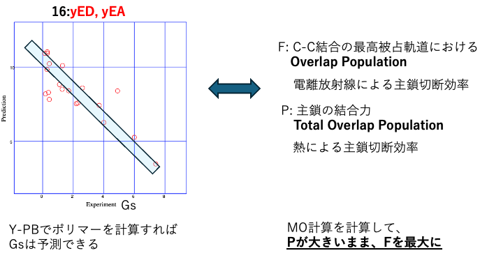
双極子モーメントと最小負電荷を用いて、Gsを決定係数0.89で計算できる。
RDKit計算ツールを使用すれば、同じく39種類のトポロジカルな物性値を取得できる。
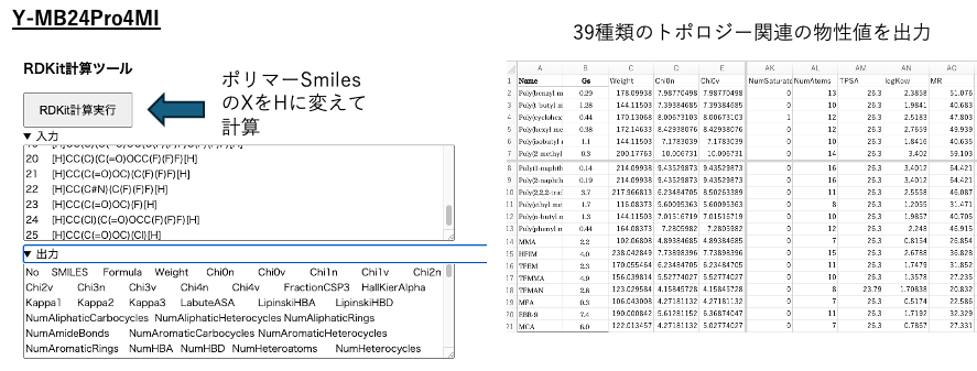
別の言い方をするなら、ポリマーSmilesを使えば、ワンストップで多角的な評価を即座に行うことができる。
これは重要な点だ。コンピュータ計算のみを用いてレジストポリマーを設計しようとする。たとえ高い相関係数を得たとしても(私の25年の経験に基づけば)、そのデータはビッグデータとは言えない。データ量が増えると、推算結果が一致しなくなる事が多い。多くの論文が大々的に発表されるが、しばしば消えていく。
私がこの分野で25年以上研究者として生き残れてきた理由は、密かにこうした多面的な評価を行い、どの列や数値を使っても結論が変わらないと確信できるまでデータを微調整してきたからだ。
多くの研究者は、分子軌道計算こそがMIにおける唯一の選択肢だと主張する。
分子軌道計算ならどんな高分子でも計算でき、化学の知識が浅くてもデータを収集し、データサイエンス風の作業を比較的短期間でこなせる。まあ、あと25年生き延びられることを願うしかないだろう。
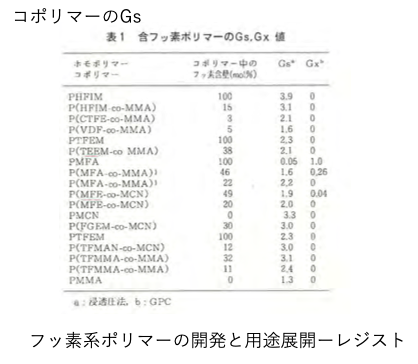
さらにこれらの高分子は単独で使用されることは稀だ。例えば共重合体として使用した場合のGs値が文献に記載されている。
現時点で、pirikaは大きな優位性を持っている。
私はもともと高分子化学に携わり、重合シミュレータ(POSEIDON)を開発した。
これにより、あらゆるモノマー組成の重合体のモノマーの並び方を分析することが可能になる。
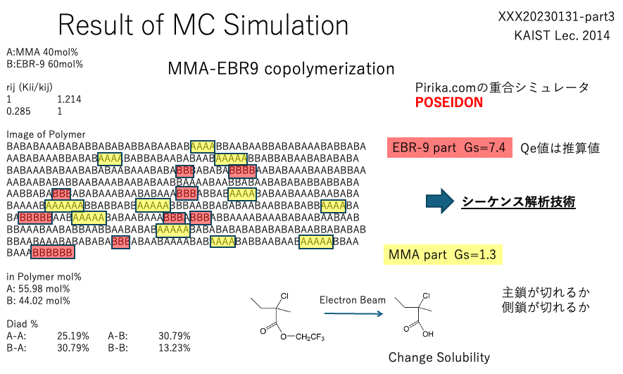
シーケンス解析にはモノマーの反応性比かQe値が必要だ。
私は分子構造からQe値を予測し、実験結果からQe値を決定するプログラムを作成した。
これらのポリマー用ツールを一つのパッケージにした。
Copyright pirika.com since 1999-
Mail: yamahiroXpirika.com (Xを@に置き換えてください)
メールの件名は[pirika]で始め